Interactions and Simple Slopes
Interactions
- Interactions have the same meaning they did in ANOVA
- there is a synergistic effect between two variables
- However now we can examine interactions between continuous variables
- Additive Effects:
\[Y = B_1X + B_2Z + B_0\]
- Interactive Effects: \[Y = B_1X + B_2Z + B_3XZ + B_0\]
Example of Interaction
- DV: Reading Speed, IVs: Age + IQ
- Simulation: \(Y = 3X + .2Z + .4XZ +100 +\epsilon\)
- So what we mean is: \(ReadingSpeed = 3*Age
+ .2*IQ + .4*Age*IQ +100 +Noise\)
- Set age to be uniform distribution between 7-17
- Set IQ to be normal, \(M\)=100 and \(S\)=15
- Set \(\epsilon\) = 15 (normal distribution of noise)
- Note: For our regression simulation to match our equation, we should center our X and Z variables first, but we will save out the raw score
set.seed(42)
n <- 200
# Uniform distribution of Ages
X <- runif(n, 7, 17)
Xc<-scale(X,scale=F)
# normal distrobution of IQ (100 +-15)
Z <- rnorm(n, 100, 15)
Zc<-scale(Z,scale=F)
# Our equation to  create Y
Y <- 3*Xc + .2*Zc + .4*Xc*Zc +100 + rnorm(n, sd=15)
#Built our data frame
Reading.Data<-data.frame(Age=X,IQ=Z,ReadingSpeed=Y)
Scatterplot & correlate our predictors
- We will use a useful diagnostic tool (GGally)
- We will visualize the density, scatterplot and correlation all at once
library(GGally)
DiagPlot <- ggpairs(Reading.Data,
              lower = list(continuous = "smooth"))
DiagPlot
- Predictors have some heteroskedastic issues, but the correlations seem to make sense
Let’s test for an interaction
- Center your variables
- Model 1: Examine a main-effects model (X + Z) [not necessary but useful]
- Model 2: Examine a main-effects + Interaction model (X + Z + X:Z)
- Note: You can simply code it as X*Z in r, as it will automatically do (X + Z + X:Z)
#Center
Reading.Data$Age.C<-scale(Reading.Data$Age, center = TRUE, scale = FALSE)[,]
Reading.Data$IQ.C<-scale(Reading.Data$IQ, center = TRUE, scale = FALSE)[,]
# Regressions
Centered.Read.1<-lm(ReadingSpeed~Age.C+IQ.C,Reading.Data)
Centered.Read.2<-lm(ReadingSpeed~Age.C*IQ.C,Reading.Data)
# Show results
library(stargazer)
stargazer(Centered.Read.1,Centered.Read.2,type="html",
          column.labels = c("Main Effects", "Interaction"),
          intercept.bottom = FALSE, single.row=TRUE,
notes.append = FALSE, header=FALSE)| Dependent variable: | ||
| ReadingSpeed | ||
| Main Effects | Interaction | |
| (1) | (2) | |
| Constant | 99.441*** (1.616) | 99.363*** (1.009) |
| Age.C | 2.287*** (0.555) | 2.412*** (0.346) |
| IQ.C | 0.213* (0.112) | 0.234*** (0.070) |
| Age.C:IQ.C | 0.402*** (0.023) | |
| Observations | 200 | 200 |
| R2 | 0.095 | 0.649 |
| Adjusted R2 | 0.086 | 0.644 |
| Residual Std. Error | 22.858 (df = 197) | 14.267 (df = 196) |
| F Statistic | 10.326*** (df = 2; 197) | 120.907*** (df = 3; 196) |
| Note: | p<0.1; p<0.05; p<0.01 | |
- Also, change in \(R^2\) is significant, as we might expect
ChangeInR<-anova(Centered.Read.1,Centered.Read.2)
knitr::kable(ChangeInR, digits=4)| Res.Df | RSS | Df | Sum of Sq | F | Pr(>F) |
|---|---|---|---|---|---|
| 197 | 102930.36 | NA | NA | NA | NA |
| 196 | 39893.42 | 1 | 63036.93 | 309.7062 | 0 |
Examine residuals
- Main Effects Model
library(ggfortify)
autoplot(Centered.Read.1, which = 1:2, label.size = 1) + theme_bw()
- Interactions Model
autoplot(Centered.Read.2, which = 1:2, label.size = 1) + theme_bw()
Understanding the Interaction
- Let’s examine a 3d scatter plot of the raw data and plot against it the predicted results of each model (additive and interaction model)
- Once we have a “model” of the data, we can generate predictions for
all possible Ages at every possible IQ
(within the absolute boundary limits for our data)
- With 2 predictors that generates a “3D surface plane.”
- You go past 2 predictors with these types of plots
- With 2 predictors that generates a “3D surface plane.”
- Let’s examine Model 1 (additive effects) as a 3D scatter/surface
plot
- Scatter dots = Raw data points
- Surface = Model 1 Predicted Results
- How well does the surface fit the dots?
- Let’s examine Model 2 (interaction effects) as a 3d scatter/surface
plot
- Scatter dots = Raw data points
- Surface = Model 2 Predicted Results
- How well does the surface fit the dots?
How visualize this for Papers?
- Well, there are some options
- We can do our fancy-pants surface plot, but that is hard to put into a paper
- More common this is to examine slope of one factor at different levels of the other (Simple Slopes)
- What we need to decide is at which levels
Hand picking
- Manually select the what levels of each you are going to examine
- For tracking values of interest
- here I picked -3 to 3 for age (mix and max) and -15, 0 15 for IQ (theoretical 1 SD and mean)
library(effects)
Inter.1a<-effect(c("Age.C*IQ.C"), Centered.Read.2,
                           xlevels=list(Age.C=seq(-3,3, 1),
                                        IQ.C=c(-15,0,15)))
knitr::kable(summary(Inter.1a)$effect, digits=4)
plot(Inter.1a, multiline = TRUE)| -15 | 0 | 15 | |
|---|---|---|---|
| -3 | 106.7108 | 92.1283 | 77.5458 |
| -2 | 103.0896 | 94.5398 | 85.9900 |
| -1 | 99.4684 | 96.9513 | 94.4343 |
| 0 | 95.8471 | 99.3629 | 102.8786 |
| 1 | 92.2259 | 101.7744 | 111.3229 |
| 2 | 88.6047 | 104.1859 | 119.7671 |
| 3 | 84.9835 | 106.5974 | 128.2114 |

Quantile
- Examine the levels based on quantiles (bins based on probability)
- We will do this into 5 equal bins based on probability cut-offs
- Does not assume normality for IV
IQ.Quantile<-quantile(Reading.Data$IQ.C,probs=c(0,.25,.50,.75,1))
IQ.Quantile<-round(IQ.Quantile,2)

Inter.1b<-effect(c("Age.C*IQ.C"), Centered.Read.2,
                 xlevels=list(Age.C=seq(-3,3, 1),
                              IQ.C=IQ.Quantile))
plot(Inter.1b, multiline = TRUE)
Based on the SD
- We select 3 values: \(M-1SD\), \(M\), \(M+1SD\)
- Not it does not have to be 1 SD, it can be 1.5 ,2 or 3
- Assumes normality for IV
IQ.SD<-c(mean(Reading.Data$IQ.C)-sd(Reading.Data$IQ.C),
         mean(Reading.Data$IQ.C),
         mean(Reading.Data$IQ.C)+sd(Reading.Data$IQ.C))
IQ.SD<-round(IQ.SD,2)

Inter.1c<-effect(c("Age.C*IQ.C"), Centered.Read.2,
                 xlevels=list(Age.C=seq(-3,3, 1),
                              IQ.C=IQ.SD))
plot(Inter.1c, multiline = TRUE)
Why center your IVs?
- The center of each IV represents the mean of that IV
- Thus when you interact them \(X*Z\), that means \(0*0 = 0\)
- Also, this can reduce multicollinearity issues
- This is because if \(X*Z\) creates a line, it means you have added a new predictor (XZ) that strongly correlates with X and Z
X<-c(0,2,4,6,8,10)
Z<-c(0,2,4,6,8,10)
XZ<-X*Z
plot(XZ)
- Correlations: \(r_{x,z}\) = 1, \(r_{x,xz}\) = 0.96, \(r_{z,xz}\) = 0.96 -But if you center them, now you will make a U-shaped interaction which will be orthogonal to X and Z!
X.C<-scale(X, center = TRUE, scale = FALSE)[,]
Z.C<-scale(Z, center = TRUE, scale = FALSE)[,]
XZ.C<-X.C*Z.C
plot(XZ.C)
Correlations: \(r_{x_c,z_c}\) = 1, \(r_{x_c,xz_c}\) = 0, \(r_{z_c,xz_c}\) = 0
Let’s apply this to our class example
See below where I manually multiply the values and you can see a very strong positive slope
Left = Raw Score, Right plot = Centered Score


Let’s run an uncentered regression
- as you can see the terms have changed from centered models
Uncentered.Read.1<-lm(ReadingSpeed~IQ+Age,Reading.Data)
Uncentered.Read.2<-lm(ReadingSpeed~IQ*Age,Reading.Data)| Dependent variable: | ||
| ReadingSpeed | ||
| Main Effects | Interaction | |
| (1) | (2) | |
| Constant | 50.328*** (13.134) | 534.570*** (28.711) |
| IQ | 0.213* (0.112) | -4.681*** (0.287) |
| Age | 2.287*** (0.555) | -37.512*** (2.288) |
| IQ:Age | 0.402*** (0.023) | |
| Observations | 200 | 200 |
| R2 | 0.095 | 0.649 |
| Adjusted R2 | 0.086 | 0.644 |
| Residual Std. Error | 22.858 (df = 197) | 14.267 (df = 196) |
| F Statistic | 10.326*** (df = 2; 197) | 120.907*** (df = 3; 196) |
| Note: | p<0.1; p<0.05; p<0.01 | |
Multicollinearity of the Interaction
- Multicollinearity of the uncentered model
vif(Uncentered.Read.2)## IQ Age IQ:Age
## 16.70086 43.64111 59.58237- We lost our main effect of Age as the variances got all inflated
- We did not have this problem in the centered model
vif(Centered.Read.2)## Age.C IQ.C Age.C:IQ.C
## 1.000440 1.000316 1.000716- Note: Its OK to plot the uncentered version, but run the analysis on the centered data
Testing Simple Slopes
- The goal here is to figure out when the slope at a given level of another variable is different from zero
- We chop up the interaction at specific places as we did with the interactions plots (-1 SD, M, +1 SD) on the moderating variable (a third variable that affects the strength of the relationship between a dependent and independent variable)
- Next, we test the slopes on the predictor variable (IV of main interest)
- Example: Performance on a task, predicted by Level of training, moderated by how hard the challenge is
Example of Interaction
- DV: Performance, IVs: Training (X) + Challenge (Z)
- Simulation: \(Y = 2.2X + 2.46Z + .75XZ +16
+\epsilon\)
- Set Training to be uniform distribution between -10 to 10
- Set Challenge to be normal, \(M\)=0 and \(S\)=15
- Set \(\epsilon\) = 50 (normal distribution of noise)
- Note: For our regression simulation we will set means to about zero (so are not forced to center them)
set.seed(42)
# 250 people
n <- 250
#Training (low to high)
X <- runif(n, -10, 10)
# normal distribution of Challenge Difficulty
Z <- rnorm(n, 0, 15)
# Our equation to  create Y
Y <- 2.2*X + 2.46*Z + .75*X*Z + 16 + rnorm(n, sd=50)
#Built our data frame
Skill.Data<-data.frame(Training=X,Challenge=Z,Performance=Y)
#run our regression
Skill.Model.1<-lm(Performance~Training+Challenge,Skill.Data)
Skill.Model.2<-lm(Performance~Training*Challenge,Skill.Data)
| Dependent variable: | ||
| Performance | ||
| Main Effects | Interaction | |
| (1) | (2) | |
| Constant | 14.238*** (4.909) | 16.173*** (3.268) |
| Training | 0.895 (0.843) | 1.542*** (0.562) |
| Challenge | 2.855*** (0.354) | 2.600*** (0.236) |
| Training:Challenge | 0.762*** (0.043) | |
| Observations | 250 | 250 |
| R2 | 0.210 | 0.652 |
| Adjusted R2 | 0.204 | 0.648 |
| Residual Std. Error | 77.510 (df = 247) | 51.571 (df = 246) |
| F Statistic | 32.867*** (df = 2; 247) | 153.486*** (df = 3; 246) |
| Note: | p<0.1; p<0.05; p<0.01 | |
Plotting
- We will use the
rockchalklibrary to visualize our interaction and test our simple slopes
library(rockchalk)
m1ps <- plotSlopes(Skill.Model.2, modx = "Challenge", plotx = "Training", n=3, modxVals="std.dev")
m1psts <- testSlopes(m1ps)
round(m1psts$hypotests,4)
## Values of Challenge OUTSIDE this interval:
## lo hi
## -3.5050807 -0.5730182
## cause the slope of (b1 + b2*Challenge)Training to be statistically significant
## "Challenge" slope Std. Error t value Pr(>|t|)
## (m-sd) -14.50 -9.5013 0.8131 -11.6848 0.0000
## (m) -0.61 1.0771 0.5611 1.9196 0.0561
## (m+sd) 13.28 11.6554 0.8282 14.0737 0.0000
- We see the slope at the mean is not significant,
- The +1SD and -1SD are significant, this is what is driving the interaction
- Well trained people at low levels of challenge get worse with more training, while high levels of challenge with more training get better
- The bonus using rockchalk is that you can change the number of lines (change \(n=3\)) you want to see or you can test quantiles as well (change modxVals=“quantile”)
m1pQ <- plotSlopes(Skill.Model.2, modx = "Challenge", plotx = "Training", n=5, modxVals="quantile")
m1pQts <- testSlopes(m1pQ)
round(m1pQts$hypotests,4)
## Values of Challenge OUTSIDE this interval:
## lo hi
## -3.5050807 -0.5730182
## cause the slope of (b1 + b2*Challenge)Training to be statistically significant
## "Challenge" slope Std. Error t value Pr(>|t|)
## 0% -40.4989 -29.3016 1.7993 -16.2847 0.0000
## 25% -10.5190 -6.4694 0.6990 -9.2555 0.0000
## 50% -0.7985 0.9335 0.5610 1.6640 0.0974
## 75% 8.8382 8.2726 0.6994 11.8278 0.0000
## 100% 36.8939 29.6394 1.7214 17.2183 0.0000
Notes
- You often don’t need to run the t-tests on the simple slopes, but they can useful to test very specific hypotheses
- You can run simple slopes analysis on three-way interactions, but let’s leave that aside for now as you would have to use a different R-package
Non-Linear interactions
- You can have non-linear terms interacting with other linear and non-linear terms
- Example: Quit smoking, X = Fear of your health, Z = moderated by Self-Efficacy for quitting
Example of Polynomial Interaction
- DV: Quit smoking, IVs: Fear (X) + Self-Efficacy (Z)
- Simulation: \(Y = -.18X - .15X^2 + Z +
.16XZ + .07X^2Z +20 +\epsilon\)
- Set Fear of your health to be uniform distribution between 1 to 9 (centered)
- Set Self-Efficacy to be normal, \(M\)=0 and \(S\)=15
- Set \(\epsilon\) = 10 (normal distribution of noise)
set.seed(42)
n <- 250
#Fear of Health
X <- scale(runif(n, 1, 9), scale=F)
#Centered Self-Efficacy
Z <- scale(runif(n, 0, 15), scale=F)
# Our equation to  create Y
Y <- -.05*X - .20*X^2 + .15*X*Z + .22*(X^2)*Z+ 35 + rnorm(n, sd=10)
#Built our data frame
Smoke.Data<-data.frame(Smoking=Y,Health=X,SelfEfficacy=Z)
#run our regression
Smoke.Model.1<-lm(Smoking~poly(Health,2)+SelfEfficacy,Smoke.Data)
Smoke.Model.2<-lm(Smoking~poly(Health,2)*SelfEfficacy,Smoke.Data)
Smoke.Model.1.R<-lm(Smoking~poly(Health,2, raw=T)+SelfEfficacy,Smoke.Data)
Smoke.Model.2.R<-lm(Smoking~poly(Health,2, raw=T)*SelfEfficacy,Smoke.Data)- Orthogonal Polynomials
| Dependent variable: | ||
| Smoking | ||
| Main Effects | Interaction | |
| (1) | (2) | |
| Constant | 33.263*** (0.680) | 33.493*** (0.621) |
| poly(Health, 2)1 | 1.010 (10.786) | 3.083 (9.813) |
| poly(Health, 2)2 | -9.037 (10.766) | -6.505 (9.795) |
| SelfEfficacy | 1.188*** (0.155) | 1.189*** (0.141) |
| poly(Health, 2)1:SelfEfficacy | 3.042 (2.218) | |
| poly(Health, 2)2:SelfEfficacy | 16.361*** (2.288) | |
| Observations | 250 | 250 |
| R2 | 0.197 | 0.341 |
| Adjusted R2 | 0.187 | 0.328 |
| Residual Std. Error | 10.759 (df = 246) | 9.781 (df = 244) |
| F Statistic | 20.058*** (df = 3; 246) | 25.297*** (df = 5; 244) |
| Note: | p<0.1; p<0.05; p<0.01 | |
- Power Polynomials
| Dependent variable: | ||
| Smoking | ||
| Main Effects Non-Ortho | Interaction Non-Ortho | |
| (1) | (2) | |
| Constant | 33.909*** (1.027) | 33.958*** (0.934) |
| poly(Health, 2, raw = T)1 | 0.009 (0.294) | 0.070 (0.268) |
| poly(Health, 2, raw = T)2 | -0.119 (0.142) | -0.086 (0.129) |
| SelfEfficacy | 1.188*** (0.155) | 0.020 (0.217) |
| poly(Health, 2, raw = T)1:SelfEfficacy | 0.116* (0.060) | |
| poly(Health, 2, raw = T)2:SelfEfficacy | 0.216*** (0.030) | |
| Observations | 250 | 250 |
| R2 | 0.197 | 0.341 |
| Adjusted R2 | 0.187 | 0.328 |
| Residual Std. Error | 10.759 (df = 246) | 9.781 (df = 244) |
| F Statistic | 20.058*** (df = 3; 246) | 25.297*** (df = 5; 244) |
| Note: | p<0.1; p<0.05; p<0.01 | |
- Note how different the results might look when you examine that as power polynomials
Plotting the Simple Slopes when there are Curves
- These can be done with the
effectspackage as I showed you above and last week - We will work with the orthogonal polynomial models
- or we can simply use the plotCurves function from the ‘rockchalk’ package
SmokeInterPlot <- plotCurves(Smoke.Model.2,
                             modx = "SelfEfficacy", plotx = "Health",
                             n=3,modxVals="std.dev")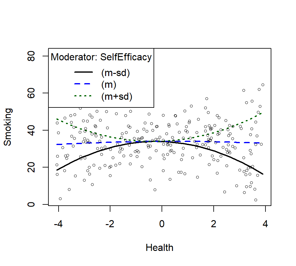
- Lets plot just the main effect (and think about what it means relative the power)
plotCurves(Smoke.Model.1, plotx = "Health")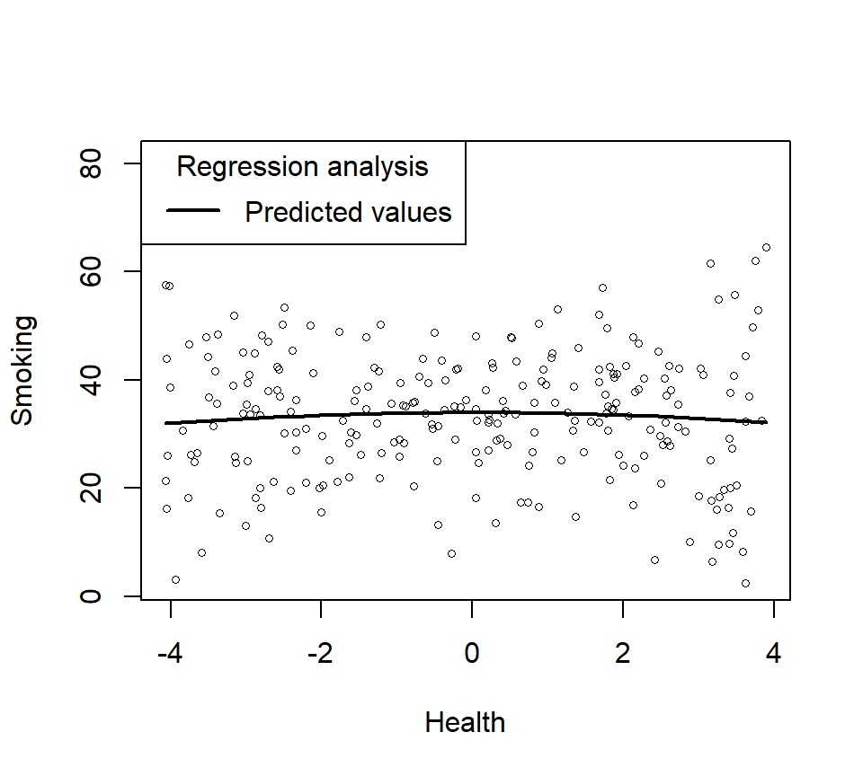
- Does not look very quadratic, does it? In other words, you cannot see the higher order effects as they can be hidden by the moderating variable
- How to find these hidden things?
- You have to test for interactions and changes in \(R^2\)
- You have to try to add higher order terms, but they should be motivated by some theory
- What if you did not know the second order term was in the model above.
Smoke.Model.1.L<-lm(Smoking~Health+SelfEfficacy,Smoke.Data)
Smoke.Model.2.L<-lm(Smoking~Health*SelfEfficacy,Smoke.Data)| Dependent variable: | ||
| Smoking | ||
| Main Effects | Interaction | |
| (1) | (2) | |
| Constant | 33.263*** (0.680) | 33.334*** (0.680) |
| Health | 0.028 (0.293) | 0.042 (0.292) |
| SelfEfficacy | 1.193*** (0.155) | 1.207*** (0.155) |
| Health:SelfEfficacy | 0.097 (0.066) | |
| Observations | 250 | 250 |
| R2 | 0.194 | 0.201 |
| Adjusted R2 | 0.188 | 0.192 |
| Residual Std. Error | 10.752 (df = 247) | 10.727 (df = 246) |
| F Statistic | 29.770*** (df = 2; 247) | 20.666*** (df = 3; 246) |
| Note: | p<0.1; p<0.05; p<0.01 | |
ChangeInR.Smoke<-anova(Smoke.Model.1.L,Smoke.Model.2.L)
knitr::kable(ChangeInR.Smoke, digits=4)| Res.Df | RSS | Df | Sum of Sq | F | Pr(>F) |
|---|---|---|---|---|---|
| 247 | 28557.09 | NA | NA | NA | NA |
| 246 | 28306.63 | 1 | 250.4599 | 2.1766 | 0.1414 |
- There is no significant interaction, but let’s plot it anyway.
- Replotting as linear interaction
SmokeInterPlot.Linear <- plotSlopes(Smoke.Model.2.L, modx = "SelfEfficacy", plotx = "Health", n=3, modxVals="std.dev")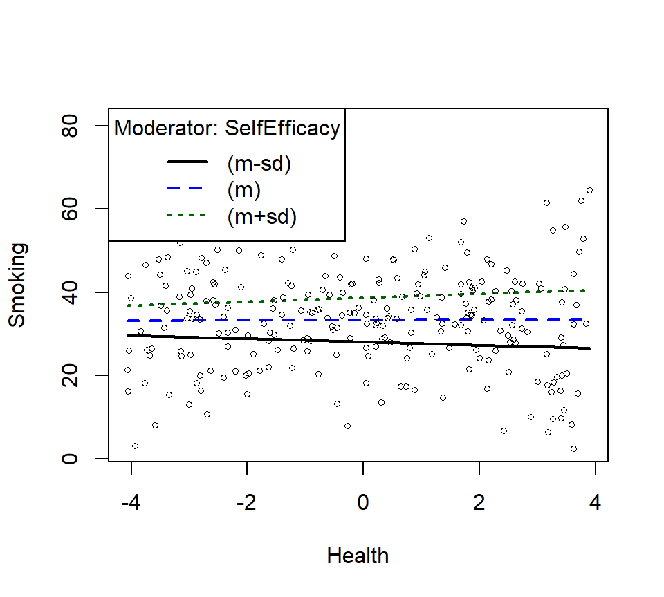
- Let’s check the change in \(R^2\) from Linear interaction model to poly interaction model now
stargazer(Smoke.Model.2.L,Smoke.Model.2,type="html",
          column.labels = c("Linear", "Poly"),
          intercept.bottom = FALSE,
          single.row=TRUE,
          notes.append = FALSE,
header=FALSE)| Dependent variable: | ||
| Smoking | ||
| Linear | Poly | |
| (1) | (2) | |
| Constant | 33.334*** (0.680) | 33.493*** (0.621) |
| Health | 0.042 (0.292) | |
| poly(Health, 2)1 | 3.083 (9.813) | |
| poly(Health, 2)2 | -6.505 (9.795) | |
| SelfEfficacy | 1.207*** (0.155) | 1.189*** (0.141) |
| Health:SelfEfficacy | 0.097 (0.066) | |
| poly(Health, 2)1:SelfEfficacy | 3.042 (2.218) | |
| poly(Health, 2)2:SelfEfficacy | 16.361*** (2.288) | |
| Observations | 250 | 250 |
| R2 | 0.201 | 0.341 |
| Adjusted R2 | 0.192 | 0.328 |
| Residual Std. Error | 10.727 (df = 246) | 9.781 (df = 244) |
| F Statistic | 20.666*** (df = 3; 246) | 25.297*** (df = 5; 244) |
| Note: | p<0.1; p<0.05; p<0.01 | |
ChangeInR.Smoke.2<-anova(Smoke.Model.2,Smoke.Model.2.L)
knitr::kable(ChangeInR.Smoke.2, digits=4)| Res.Df | RSS | Df | Sum of Sq | F | Pr(>F) |
|---|---|---|---|---|---|
| 244 | 23341.19 | NA | NA | NA | NA |
| 246 | 28306.63 | -2 | -4965.442 | 25.9534 | 0 |
Notes
- So, model with poly is a significantly better fit
- Would it change the story by much? In this case YES, but not always!
- Sometimes the improvement in fit is minor and does not change the
story
- Often ignoring the higher order term can make it easier to test simple slopes and tell a story
- However, ignoring the higher order terms can violate your assumptions when the results, let’s compare our linear vs poly models residuals
- Sometimes the improvement in fit is minor and does not change the
story
- Linear Model
autoplot(Smoke.Model.2, which = 1:2, label.size = 1) + theme_bw()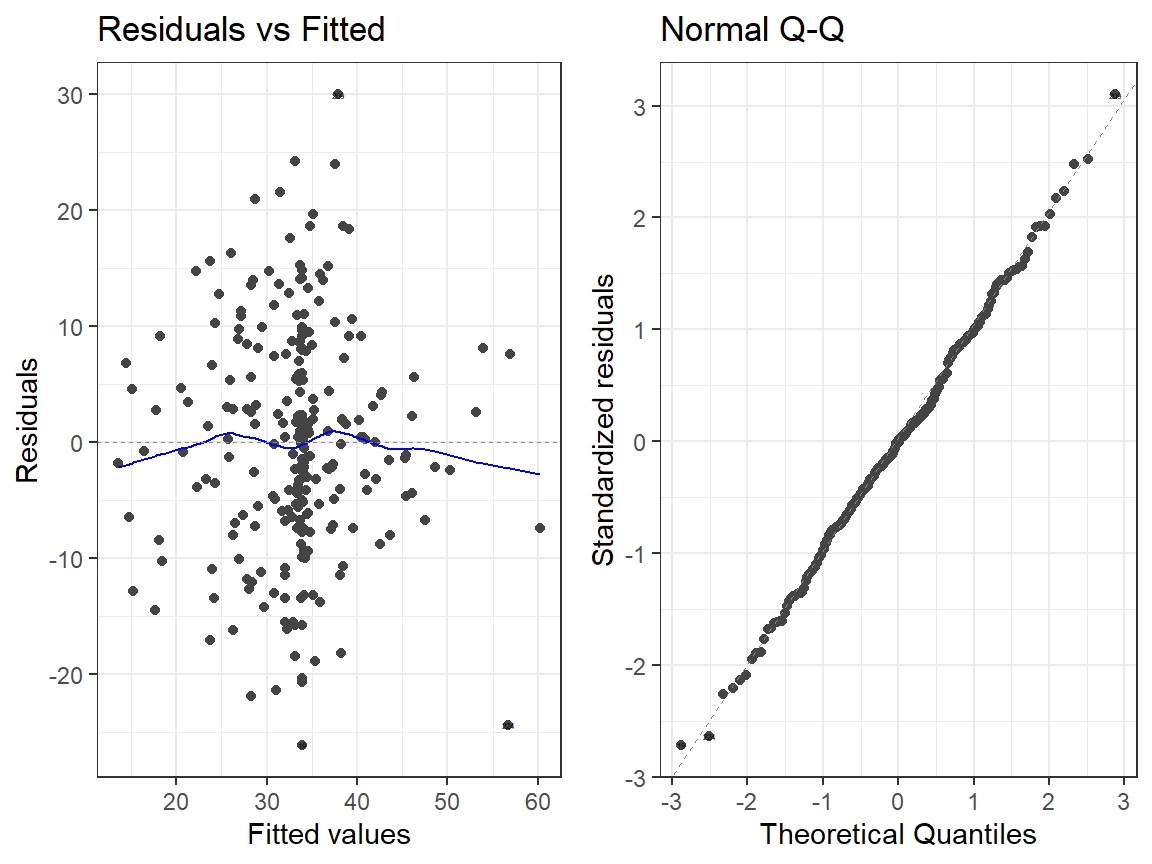
- Quadtradic Model
autoplot(Smoke.Model.2.L, which = 1:2, label.size = 1) + theme_bw()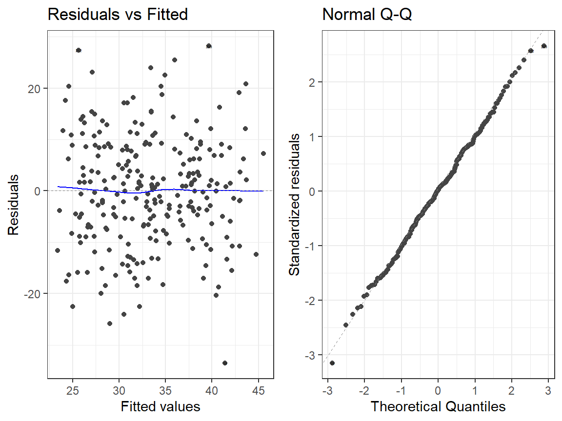
LS0tDQp0aXRsZTogJ0ludGVyYWN0aW9ucyBhbmQgU2ltcGxlIFNsb3BlcycNCm91dHB1dDoNCiAgaHRtbF9kb2N1bWVudDoNCiAgICBjb2RlX2Rvd25sb2FkOiB5ZXMNCiAgICBmb250c2l6ZTogOHB0DQogICAgaGlnaGxpZ2h0OiB0ZXh0bWF0ZQ0KICAgIG51bWJlcl9zZWN0aW9uczogbm8NCiAgICB0aGVtZTogZmxhdGx5DQogICAgdG9jOiB5ZXMNCiAgICB0b2NfZmxvYXQ6DQogICAgICBjb2xsYXBzZWQ6IG5vDQotLS0NCg0KYGBge3Igc2V0dXAsIGluY2x1ZGU9RkFMU0V9DQprbml0cjo6b3B0c19jaHVuayRzZXQoY2FjaGU9VFJVRSkNCmtuaXRyOjpvcHRzX2NodW5rJHNldChlY2hvID0gVFJVRSkgI1Nob3cgYWxsIHNjcmlwdCBieSBkZWZhdWx0DQprbml0cjo6b3B0c19jaHVuayRzZXQobWVzc2FnZSA9IEZBTFNFKSAjaGlkZSBtZXNzYWdlcyANCmtuaXRyOjpvcHRzX2NodW5rJHNldCh3YXJuaW5nID0gIEZBTFNFKSAjaGlkZSBwYWNrYWdlIHdhcm5pbmdzIA0Ka25pdHI6Om9wdHNfY2h1bmskc2V0KGZpZy53aWR0aD01KSAjU2V0IGRlZmF1bHQgZmlndXJlIHNpemVzDQprbml0cjo6b3B0c19jaHVuayRzZXQoZmlnLmhlaWdodD00LjUpICNTZXQgZGVmYXVsdCBmaWd1cmUgc2l6ZXMNCmtuaXRyOjpvcHRzX2NodW5rJHNldChmaWcuYWxpZ249J2NlbnRlcicpICNTZXQgZGVmYXVsdCBmaWd1cmUNCmtuaXRyOjpvcHRzX2NodW5rJHNldChmaWcuc2hvdyA9ICJob2xkIikgI1NldCBkZWZhdWx0IGZpZ3VyZQ0Ka25pdHI6Om9wdHNfY2h1bmskc2V0KHJlc3VsdHMgPSAiaG9sZCIpICNTZXQgZGVmYXVsdCBmaWd1cmUNCmBgYA0KDQojIEludGVyYWN0aW9ucw0KLSBJbnRlcmFjdGlvbnMgaGF2ZSB0aGUgc2FtZSBtZWFuaW5nIHRoZXkgZGlkIGluIEFOT1ZBDQogICAgLSB0aGVyZSBpcyBhIHN5bmVyZ2lzdGljIGVmZmVjdCBiZXR3ZWVuIHR3byB2YXJpYWJsZXMNCiAgICAtIEhvd2V2ZXIgbm93IHdlIGNhbiBleGFtaW5lIGludGVyYWN0aW9ucyBiZXR3ZWVuIGNvbnRpbnVvdXMgdmFyaWFibGVzDQotIEFkZGl0aXZlIEVmZmVjdHM6DQoNCiQkWSA9IEJfMVggKyBCXzJaICsgQl8wJCQNCg0KLSBJbnRlcmFjdGl2ZSBFZmZlY3RzOiANCiQkWSA9IEJfMVggKyBCXzJaICsgQl8zWFogKyBCXzAkJA0KDQoNCiMjIEV4YW1wbGUgb2YgSW50ZXJhY3Rpb24NCi0gRFY6IFJlYWRpbmcgU3BlZWQsIElWczogQWdlICsgSVEgDQotIFNpbXVsYXRpb246ICRZID0gM1ggKyAuMlogKyAuNFhaICsxMDAgK1xlcHNpbG9uJA0KLSBTbyB3aGF0IHdlIG1lYW4gaXM6ICRSZWFkaW5nU3BlZWQgPSAzKkFnZSArIC4yKklRICsgLjQqQWdlKklRICsxMDAgK05vaXNlJA0KICAgIC0gU2V0IGFnZSB0byBiZSB1bmlmb3JtIGRpc3RyaWJ1dGlvbiBiZXR3ZWVuIDctMTcgDQogICAgLSBTZXQgSVEgdG8gYmUgbm9ybWFsLCAkTSQ9MTAwIGFuZCAkUyQ9MTUNCiAgICAtIFNldCAkXGVwc2lsb24kID0gMTUgKG5vcm1hbCBkaXN0cmlidXRpb24gb2Ygbm9pc2UpDQogICAgLSBOb3RlOiBGb3Igb3VyIHJlZ3Jlc3Npb24gc2ltdWxhdGlvbiB0byBtYXRjaCBvdXIgZXF1YXRpb24sIHdlIHNob3VsZCBjZW50ZXIgb3VyIFggYW5kIFogdmFyaWFibGVzIGZpcnN0LCBidXQgd2Ugd2lsbCBzYXZlIG91dCB0aGUgcmF3IHNjb3JlIA0KYGBge3IsIGVjaG89VFJVRSwgd2FybmluZz1GQUxTRX0NCnNldC5zZWVkKDQyKQ0KbiA8LSAyMDANCiMgVW5pZm9ybSBkaXN0cmlidXRpb24gb2YgQWdlcyANClggPC0gcnVuaWYobiwgNywgMTcpDQpYYzwtc2NhbGUoWCxzY2FsZT1GKQ0KIyBub3JtYWwgZGlzdHJvYnV0aW9uIG9mIElRICgxMDAgKy0xNSkgDQpaIDwtIHJub3JtKG4sIDEwMCwgMTUpDQpaYzwtc2NhbGUoWixzY2FsZT1GKQ0KIyBPdXIgZXF1YXRpb24gdG8gIGNyZWF0ZSBZDQpZIDwtIDMqWGMgKyAuMipaYyArIC40KlhjKlpjICsxMDAgKyBybm9ybShuLCBzZD0xNSkNCiNCdWlsdCBvdXIgZGF0YSBmcmFtZQ0KUmVhZGluZy5EYXRhPC1kYXRhLmZyYW1lKEFnZT1YLElRPVosUmVhZGluZ1NwZWVkPVkpDQpgYGANCg0KIyMgU2NhdHRlcnBsb3QgJiBjb3JyZWxhdGUgb3VyIHByZWRpY3RvcnMNCi0gV2Ugd2lsbCB1c2UgYSB1c2VmdWwgZGlhZ25vc3RpYyB0b29sIChHR2FsbHkpDQotIFdlIHdpbGwgdmlzdWFsaXplIHRoZSBkZW5zaXR5LCBzY2F0dGVycGxvdCBhbmQgY29ycmVsYXRpb24gYWxsIGF0IG9uY2UNCg0KYGBge3IsZmlnLndpZHRoPTQuNSxmaWcuaGVpZ2h0PTQuNX0NCmxpYnJhcnkoR0dhbGx5KQ0KRGlhZ1Bsb3QgPC0gZ2dwYWlycyhSZWFkaW5nLkRhdGEsICANCiAgICAgICAgICAgICAgbG93ZXIgPSBsaXN0KGNvbnRpbnVvdXMgPSAic21vb3RoIikpDQpEaWFnUGxvdA0KYGBgDQoNCi0gUHJlZGljdG9ycyBoYXZlIHNvbWUgaGV0ZXJvc2tlZGFzdGljIGlzc3VlcywgYnV0IHRoZSBjb3JyZWxhdGlvbnMgc2VlbSB0byBtYWtlIHNlbnNlDQoNCg0KIyMgTGV0J3MgdGVzdCBmb3IgYW4gaW50ZXJhY3Rpb24NCjEuIENlbnRlciB5b3VyIHZhcmlhYmxlcw0KMi4gTW9kZWwgMTogRXhhbWluZSBhIG1haW4tZWZmZWN0cyBtb2RlbCAoWCArIFopIFtub3QgbmVjZXNzYXJ5IGJ1dCB1c2VmdWxdDQozLiBNb2RlbCAyOiBFeGFtaW5lIGEgbWFpbi1lZmZlY3RzICsgSW50ZXJhY3Rpb24gbW9kZWwgKFggKyBaICsgWDpaKQ0KDQotIE5vdGU6IFlvdSBjYW4gc2ltcGx5IGNvZGUgaXQgYXMgWCpaIGluIHIsIGFzIGl0IHdpbGwgYXV0b21hdGljYWxseSBkbyAoWCArIFogKyBYOlopDQoNCmBgYHtyLCBlY2hvPVRSVUUsIHJlc3VsdHM9J2FzaXMnfQ0KI0NlbnRlcg0KUmVhZGluZy5EYXRhJEFnZS5DPC1zY2FsZShSZWFkaW5nLkRhdGEkQWdlLCBjZW50ZXIgPSBUUlVFLCBzY2FsZSA9IEZBTFNFKVssXQ0KUmVhZGluZy5EYXRhJElRLkM8LXNjYWxlKFJlYWRpbmcuRGF0YSRJUSwgY2VudGVyID0gVFJVRSwgc2NhbGUgPSBGQUxTRSlbLF0NCiMgUmVncmVzc2lvbnMNCkNlbnRlcmVkLlJlYWQuMTwtbG0oUmVhZGluZ1NwZWVkfkFnZS5DK0lRLkMsUmVhZGluZy5EYXRhKQ0KQ2VudGVyZWQuUmVhZC4yPC1sbShSZWFkaW5nU3BlZWR+QWdlLkMqSVEuQyxSZWFkaW5nLkRhdGEpDQojIFNob3cgcmVzdWx0cw0KbGlicmFyeShzdGFyZ2F6ZXIpDQpzdGFyZ2F6ZXIoQ2VudGVyZWQuUmVhZC4xLENlbnRlcmVkLlJlYWQuMix0eXBlPSJodG1sIiwNCiAgICAgICAgICBjb2x1bW4ubGFiZWxzID0gYygiTWFpbiBFZmZlY3RzIiwgIkludGVyYWN0aW9uIiksDQogICAgICAgICAgaW50ZXJjZXB0LmJvdHRvbSA9IEZBTFNFLCBzaW5nbGUucm93PVRSVUUsIA0KICAgICAgICAgIG5vdGVzLmFwcGVuZCA9IEZBTFNFLCBoZWFkZXI9RkFMU0UpDQpgYGANCg0KLSBBbHNvLCBjaGFuZ2UgaW4gJFJeMiQgaXMgc2lnbmlmaWNhbnQsIGFzIHdlIG1pZ2h0IGV4cGVjdA0KDQpgYGB7cn0NCkNoYW5nZUluUjwtYW5vdmEoQ2VudGVyZWQuUmVhZC4xLENlbnRlcmVkLlJlYWQuMikNCmtuaXRyOjprYWJsZShDaGFuZ2VJblIsIGRpZ2l0cz00KQ0KYGBgDQoNCiMjIyBFeGFtaW5lIHJlc2lkdWFscw0KLSBNYWluIEVmZmVjdHMgTW9kZWwNCmBgYHtyLCBmaWcud2lkdGg9Nn0NCmxpYnJhcnkoZ2dmb3J0aWZ5KQ0KYXV0b3Bsb3QoQ2VudGVyZWQuUmVhZC4xLCB3aGljaCA9IDE6MiwgbGFiZWwuc2l6ZSA9IDEpICsgdGhlbWVfYncoKQ0KYGBgDQoNCi0gSW50ZXJhY3Rpb25zIE1vZGVsDQoNCmBgYHtyLCBmaWcud2lkdGg9Nn0NCmF1dG9wbG90KENlbnRlcmVkLlJlYWQuMiwgd2hpY2ggPSAxOjIsIGxhYmVsLnNpemUgPSAxKSArIHRoZW1lX2J3KCkNCmBgYA0KDQojIyBVbmRlcnN0YW5kaW5nIHRoZSBJbnRlcmFjdGlvbiANCi0gTGV0J3MgZXhhbWluZSBhIDNkIHNjYXR0ZXIgcGxvdCBvZiB0aGUgcmF3IGRhdGEgYW5kIHBsb3QgYWdhaW5zdCBpdCB0aGUgcHJlZGljdGVkIHJlc3VsdHMgb2YgZWFjaCBtb2RlbCAoYWRkaXRpdmUgYW5kIGludGVyYWN0aW9uIG1vZGVsKQ0KLSBPbmNlIHdlIGhhdmUgYSAibW9kZWwiIG9mIHRoZSBkYXRhLCB3ZSBjYW4gZ2VuZXJhdGUgcHJlZGljdGlvbnMgZm9yICoqYWxsIHBvc3NpYmxlIEFnZXMqKiBhdCAqKmV2ZXJ5IHBvc3NpYmxlIElRKiogKHdpdGhpbiB0aGUgYWJzb2x1dGUgYm91bmRhcnkgbGltaXRzIGZvciBvdXIgZGF0YSkNCiAgICAtIFdpdGggMiBwcmVkaWN0b3JzIHRoYXQgZ2VuZXJhdGVzIGEgIjNEIHN1cmZhY2UgcGxhbmUuIg0KICAgICAgICAtIFlvdSBnbyBwYXN0IDIgcHJlZGljdG9ycyB3aXRoIHRoZXNlIHR5cGVzIG9mIHBsb3RzDQotIExldCdzIGV4YW1pbmUgTW9kZWwgMSAoYWRkaXRpdmUgZWZmZWN0cykgYXMgYSAzRCBzY2F0dGVyL3N1cmZhY2UgcGxvdA0KICAgIC0gU2NhdHRlciBkb3RzID0gUmF3IGRhdGEgcG9pbnRzDQogICAgLSBTdXJmYWNlID0gTW9kZWwgMSBQcmVkaWN0ZWQgUmVzdWx0cw0KICAgICAgICAtIEhvdyB3ZWxsIGRvZXMgdGhlIHN1cmZhY2UgZml0IHRoZSBkb3RzPyANCg0KYGBge3IsIGVjaG8gPSBGQUxTRX0NCmxpYnJhcnkocGxvdGx5KQ0KbGlicmFyeShkcGx5cikNClJlYWQuMTwtbG0oUmVhZGluZ1NwZWVkfkFnZStJUSxSZWFkaW5nLkRhdGEpDQpSZWFkLjI8LWxtKFJlYWRpbmdTcGVlZH5BZ2UqSVEsUmVhZGluZy5EYXRhKQ0KIyBwcmVkaWN0IG92ZXIgc2Vuc2libGUgZ3JpZCBvZiB2YWx1ZXMNCmdyYXBoX3Jlc28gPC0gLjUNCkFnZS5QTCA8LSBzZXEobWluKFJlYWRpbmcuRGF0YSRBZ2UpLCBtYXgoUmVhZGluZy5EYXRhJEFnZSksIGJ5ID0gZ3JhcGhfcmVzbykNCklRLlBMIDwtIHNlcShtaW4oUmVhZGluZy5EYXRhJElRKSwgbWF4KFJlYWRpbmcuRGF0YSRJUSksIGJ5ID0gZ3JhcGhfcmVzbykNCmQgPC0gc2V0TmFtZXMoZGF0YS5mcmFtZShleHBhbmQuZ3JpZChBZ2UuUEwsIElRLlBMKSksYygiQWdlIiwgIklRIikpDQp2YWxzMSA8LSBwcmVkaWN0KFJlYWQuMSwgbmV3ZGF0YSA9IGQpDQp2YWxzMiA8LSBwcmVkaWN0KFJlYWQuMiwgbmV3ZGF0YSA9IGQpDQojIGZvcm0gbWF0cml4IGFuZCBnaXZlIHRvIHBsb3RseQ0KbTEgPC0gbWF0cml4KHZhbHMxLCBucm93ID0gbGVuZ3RoKHVuaXF1ZShkJEFnZSkpLCBuY29sID0gbGVuZ3RoKHVuaXF1ZShkJElRKSkpDQptMiA8LSBtYXRyaXgodmFsczIsIG5yb3cgPSBsZW5ndGgodW5pcXVlKGQkQWdlKSksIG5jb2wgPSBsZW5ndGgodW5pcXVlKGQkSVEpKSkNCmBgYA0KDQpgYGB7ciwgZWNobyA9IEZBTFNFLCBmaWcud2lkdGg9NS41LGZpZy5oZWlnaHQ9NS41fQ0KcDEgPC0gcGxvdF9seShSZWFkaW5nLkRhdGEsIHggPSB+SVEsIHkgPSB+QWdlLCB6ID0gflJlYWRpbmdTcGVlZCkgJT4lDQogIGFkZF9tYXJrZXJzKG1hcmtlciA9IGxpc3Qoc2l6ZSA9IDQpKSAgJT4lIA0KICBhZGRfc3VyZmFjZSh4ID0gfklRLlBMLCB5ID0gfkFnZS5QTCwgeiA9IH5tMSxzaG93c2NhbGUgPSBGQUxTRSwgb3BhY2l0eT0uNzUpDQpwMQ0KYGBgDQoNCi0gTGV0J3MgZXhhbWluZSBNb2RlbCAyIChpbnRlcmFjdGlvbiBlZmZlY3RzKSBhcyBhIDNkIHNjYXR0ZXIvc3VyZmFjZSBwbG90DQogICAgLSBTY2F0dGVyIGRvdHMgPSBSYXcgZGF0YSBwb2ludHMNCiAgICAtIFN1cmZhY2UgPSBNb2RlbCAyIFByZWRpY3RlZCBSZXN1bHRzDQogICAgICAgIC0gSG93IHdlbGwgZG9lcyB0aGUgc3VyZmFjZSBmaXQgdGhlIGRvdHM/IA0KDQpgYGB7ciwgZWNobyA9IEZBTFNFLCBmaWcud2lkdGg9NS41LGZpZy5oZWlnaHQ9NS41fQ0KcDIgPC0gcGxvdF9seShSZWFkaW5nLkRhdGEsIHggPSB+SVEsIHkgPSB+QWdlLCB6ID0gflJlYWRpbmdTcGVlZCkgJT4lDQogIGFkZF9tYXJrZXJzKG1hcmtlciA9IGxpc3Qoc2l6ZSA9IDQpKSAgJT4lIA0KICBhZGRfc3VyZmFjZSh4ID0gfklRLlBMLCB5ID0gfkFnZS5QTCwgeiA9IH5tMixzaG93c2NhbGUgPSBGQUxTRSwgb3BhY2l0eT0uNzUpDQpwMg0KYGBgDQoNCg0KIyMgSG93IHZpc3VhbGl6ZSB0aGlzIGZvciBQYXBlcnM/DQotIFdlbGwsIHRoZXJlIGFyZSBzb21lIG9wdGlvbnMNCi0gV2UgY2FuIGRvIG91ciBmYW5jeS1wYW50cyBzdXJmYWNlIHBsb3QsIGJ1dCB0aGF0IGlzIGhhcmQgdG8gcHV0IGludG8gYSBwYXBlcg0KLSBNb3JlIGNvbW1vbiB0aGlzIGlzIHRvIGV4YW1pbmUgc2xvcGUgb2Ygb25lIGZhY3RvciBhdCBkaWZmZXJlbnQgbGV2ZWxzIG9mIHRoZSBvdGhlciAoU2ltcGxlIFNsb3BlcykgDQotIFdoYXQgd2UgbmVlZCB0byBkZWNpZGUgaXMgYXQgd2hpY2ggbGV2ZWxzDQoNCiMjIyBIYW5kIHBpY2tpbmcNCi0gTWFudWFsbHkgc2VsZWN0IHRoZSB3aGF0IGxldmVscyBvZiBlYWNoIHlvdSBhcmUgZ29pbmcgdG8gZXhhbWluZQ0KLSBGb3IgdHJhY2tpbmcgdmFsdWVzIG9mIGludGVyZXN0DQotIGhlcmUgSSBwaWNrZWQgLTMgdG8gMyBmb3IgYWdlIChtaXggYW5kIG1heCkgYW5kIC0xNSwgMCAxNSBmb3IgSVEgKHRoZW9yZXRpY2FsIDEgU0QgYW5kIG1lYW4pDQoNCmBgYHtyfQ0KbGlicmFyeShlZmZlY3RzKQ0KSW50ZXIuMWE8LWVmZmVjdChjKCJBZ2UuQypJUS5DIiksIENlbnRlcmVkLlJlYWQuMiwNCiAgICAgICAgICAgICAgICAgICAgICAgICAgIHhsZXZlbHM9bGlzdChBZ2UuQz1zZXEoLTMsMywgMSksIA0KICAgICAgICAgICAgICAgICAgICAgICAgICAgICAgICAgICAgICAgIElRLkM9YygtMTUsMCwxNSkpKQ0KYGBgDQoNCg0KYGBge3J9DQprbml0cjo6a2FibGUoc3VtbWFyeShJbnRlci4xYSkkZWZmZWN0LCBkaWdpdHM9NCkNCnBsb3QoSW50ZXIuMWEsIG11bHRpbGluZSA9IFRSVUUpDQpgYGANCg0KIyMjIFF1YW50aWxlDQotIEV4YW1pbmUgdGhlIGxldmVscyBiYXNlZCBvbiBxdWFudGlsZXMgKGJpbnMgYmFzZWQgb24gcHJvYmFiaWxpdHkpDQotIFdlIHdpbGwgZG8gdGhpcyBpbnRvIDUgZXF1YWwgYmlucyBiYXNlZCBvbiBwcm9iYWJpbGl0eSBjdXQtb2ZmcyANCi0gRG9lcyBub3QgYXNzdW1lIG5vcm1hbGl0eSBmb3IgSVYNCg0KYGBge3J9DQpJUS5RdWFudGlsZTwtcXVhbnRpbGUoUmVhZGluZy5EYXRhJElRLkMscHJvYnM9YygwLC4yNSwuNTAsLjc1LDEpKQ0KSVEuUXVhbnRpbGU8LXJvdW5kKElRLlF1YW50aWxlLDIpDQoNCkludGVyLjFiPC1lZmZlY3QoYygiQWdlLkMqSVEuQyIpLCBDZW50ZXJlZC5SZWFkLjIsDQogICAgICAgICAgICAgICAgIHhsZXZlbHM9bGlzdChBZ2UuQz1zZXEoLTMsMywgMSksIA0KICAgICAgICAgICAgICAgICAgICAgICAgICAgICAgSVEuQz1JUS5RdWFudGlsZSkpDQpwbG90KEludGVyLjFiLCBtdWx0aWxpbmUgPSBUUlVFKQ0KYGBgDQoNCiMjIyBCYXNlZCBvbiB0aGUgU0QgDQotIFdlIHNlbGVjdCAzIHZhbHVlczogJE0tMVNEJCwgJE0kLCAkTSsxU0QkDQotIE5vdCBpdCBkb2VzIG5vdCBoYXZlIHRvIGJlIDEgU0QsIGl0IGNhbiBiZSAxLjUgLDIgb3IgMw0KLSBBc3N1bWVzIG5vcm1hbGl0eSBmb3IgSVYNCg0KYGBge3J9DQpJUS5TRDwtYyhtZWFuKFJlYWRpbmcuRGF0YSRJUS5DKS1zZChSZWFkaW5nLkRhdGEkSVEuQyksDQogICAgICAgICBtZWFuKFJlYWRpbmcuRGF0YSRJUS5DKSwNCiAgICAgICAgIG1lYW4oUmVhZGluZy5EYXRhJElRLkMpK3NkKFJlYWRpbmcuRGF0YSRJUS5DKSkNCklRLlNEPC1yb3VuZChJUS5TRCwyKQ0KDQpJbnRlci4xYzwtZWZmZWN0KGMoIkFnZS5DKklRLkMiKSwgQ2VudGVyZWQuUmVhZC4yLA0KICAgICAgICAgICAgICAgICB4bGV2ZWxzPWxpc3QoQWdlLkM9c2VxKC0zLDMsIDEpLCANCiAgICAgICAgICAgICAgICAgICAgICAgICAgICAgIElRLkM9SVEuU0QpKQ0KcGxvdChJbnRlci4xYywgbXVsdGlsaW5lID0gVFJVRSkNCmBgYA0KDQojIyBXaHkgY2VudGVyIHlvdXIgSVZzPw0KLSBUaGUgY2VudGVyIG9mIGVhY2ggSVYgcmVwcmVzZW50cyB0aGUgbWVhbiBvZiB0aGF0IElWDQotIFRodXMgd2hlbiB5b3UgaW50ZXJhY3QgdGhlbSAkWCpaJCwgdGhhdCBtZWFucyAkMCowID0gMCQNCi0gQWxzbywgdGhpcyBjYW4gcmVkdWNlIG11bHRpY29sbGluZWFyaXR5IGlzc3Vlcw0KLSBUaGlzIGlzIGJlY2F1c2UgaWYgJFgqWiQgY3JlYXRlcyBhIGxpbmUsIGl0IG1lYW5zIHlvdSBoYXZlIGFkZGVkIGEgbmV3IHByZWRpY3RvciAoWFopIHRoYXQgc3Ryb25nbHkgY29ycmVsYXRlcyB3aXRoIFggYW5kIFoNCg0KYGBge3J9DQpYPC1jKDAsMiw0LDYsOCwxMCkNClo8LWMoMCwyLDQsNiw4LDEwKQ0KWFo8LVgqWg0KcGxvdChYWikNCmBgYA0KDQotIENvcnJlbGF0aW9uczogJHJfe3gsen0kID0gYHIgcm91bmQoY29yKFgsWiksMilgLCAkcl97eCx4en0kID0gYHIgcm91bmQoY29yKFgsWFopLDIpYCwgJHJfe3oseHp9JCA9IGByIHJvdW5kKGNvcihaLFhaKSwyKWANCi1CdXQgaWYgeW91IGNlbnRlciB0aGVtLCBub3cgeW91IHdpbGwgbWFrZSBhIFUtc2hhcGVkIGludGVyYWN0aW9uIHdoaWNoIHdpbGwgYmUgb3J0aG9nb25hbCB0byBYIGFuZCBaIQ0KDQpgYGB7ciwgZWNobz1UUlVFLCB3YXJuaW5nPUZBTFNFfQ0KWC5DPC1zY2FsZShYLCBjZW50ZXIgPSBUUlVFLCBzY2FsZSA9IEZBTFNFKVssXQ0KWi5DPC1zY2FsZShaLCBjZW50ZXIgPSBUUlVFLCBzY2FsZSA9IEZBTFNFKVssXQ0KWFouQzwtWC5DKlouQw0KcGxvdChYWi5DKQ0KYGBgDQoNCi0gQ29ycmVsYXRpb25zOiAkcl97eF9jLHpfY30kID0gYHIgcm91bmQoY29yKFguQyxaLkMpLDIpYCwgJHJfe3hfYyx4el9jfSQgPSBgciByb3VuZChjb3IoWC5DLFhaLkMpLDIpYCwgJHJfe3pfYyx4el9jfSQgPSBgciByb3VuZChjb3IoWi5DLFhaLkMpLDIpYA0KDQotIExldCdzIGFwcGx5IHRoaXMgdG8gb3VyIGNsYXNzIGV4YW1wbGUNCi0gU2VlIGJlbG93IHdoZXJlIEkgbWFudWFsbHkgbXVsdGlwbHkgdGhlIHZhbHVlcyBhbmQgeW91IGNhbiBzZWUgYSB2ZXJ5IHN0cm9uZyBwb3NpdGl2ZSBzbG9wZQ0KLSBMZWZ0ID0gUmF3IFNjb3JlLCBSaWdodCBwbG90ID0gQ2VudGVyZWQgU2NvcmUNCg0KYGBge3IsIGVjaG89RkFMU0UsIGZpZy53aWR0aD0zLjI1LCBmaWcuaGVpZ2h0PTMuMjUsZmlnLnNob3c9J2hvbGQnLGZpZy5hbGlnbj0nY2VudGVyJ30NCmxpYnJhcnkoY2FyKQ0KUmVhZGluZy5EYXRhJEFnZS5YLklRPC1SZWFkaW5nLkRhdGEkQWdlKlJlYWRpbmcuRGF0YSRJUQ0KUmVhZGluZy5EYXRhJEFnZS5YLklRLkM8LVJlYWRpbmcuRGF0YSRBZ2UuQypSZWFkaW5nLkRhdGEkSVEuQw0Kc2NhdHRlcnBsb3QoUmVhZGluZ1NwZWVkfkFnZS5YLklRLCBkYXRhPSBSZWFkaW5nLkRhdGEsIHJlZy5saW5lPUZBTFNFLCBzbW9vdGhlcj1sb2Vzc0xpbmUpDQpzY2F0dGVycGxvdChSZWFkaW5nU3BlZWR+QWdlLlguSVEuQywgZGF0YT0gUmVhZGluZy5EYXRhLCByZWcubGluZT1GQUxTRSwgc21vb3RoZXI9bG9lc3NMaW5lKQ0KYGBgDQoNCiMjIyBMZXQncyBydW4gYW4gdW5jZW50ZXJlZCByZWdyZXNzaW9uDQotIGFzIHlvdSBjYW4gc2VlIHRoZSB0ZXJtcyBoYXZlIGNoYW5nZWQgZnJvbSBjZW50ZXJlZCBtb2RlbHMNCg0KYGBge3IsIGVjaG89VFJVRX0NClVuY2VudGVyZWQuUmVhZC4xPC1sbShSZWFkaW5nU3BlZWR+SVErQWdlLFJlYWRpbmcuRGF0YSkNClVuY2VudGVyZWQuUmVhZC4yPC1sbShSZWFkaW5nU3BlZWR+SVEqQWdlLFJlYWRpbmcuRGF0YSkNCmBgYA0KDQpgYGB7ciwgZWNobz1GQUxTRSwgcmVzdWx0cz0nYXNpcyd9DQpzdGFyZ2F6ZXIoVW5jZW50ZXJlZC5SZWFkLjEsVW5jZW50ZXJlZC5SZWFkLjIsdHlwZT0iaHRtbCIsDQogICAgICAgICAgY29sdW1uLmxhYmVscyA9IGMoIk1haW4gRWZmZWN0cyIsICJJbnRlcmFjdGlvbiIpLA0KICAgICAgICAgIGludGVyY2VwdC5ib3R0b20gPSBGQUxTRSwgc2luZ2xlLnJvdz1UUlVFLCANCiAgICAgICAgICBub3Rlcy5hcHBlbmQgPSBGQUxTRSwgaGVhZGVyPUZBTFNFKQ0KYGBgDQoNCiMjIyMgTXVsdGljb2xsaW5lYXJpdHkgb2YgdGhlIEludGVyYWN0aW9uDQotIE11bHRpY29sbGluZWFyaXR5IG9mIHRoZSB1bmNlbnRlcmVkIG1vZGVsDQoNCmBgYHtyLCBlY2hvPVRSVUUsIHdhcm5pbmc9RkFMU0V9DQp2aWYoVW5jZW50ZXJlZC5SZWFkLjIpDQpgYGANCg0KLSBXZSBsb3N0IG91ciBtYWluIGVmZmVjdCBvZiAqKkFnZSoqIGFzIHRoZSB2YXJpYW5jZXMgZ290IGFsbCBpbmZsYXRlZA0KLSBXZSBkaWQgbm90IGhhdmUgdGhpcyBwcm9ibGVtIGluIHRoZSBjZW50ZXJlZCBtb2RlbA0KDQpgYGB7ciwgZWNobz1UUlVFLCB3YXJuaW5nPUZBTFNFfQ0KdmlmKENlbnRlcmVkLlJlYWQuMikNCmBgYA0KDQotIE5vdGU6IEl0cyBPSyB0byBwbG90IHRoZSB1bmNlbnRlcmVkIHZlcnNpb24sIGJ1dCBydW4gdGhlIGFuYWx5c2lzIG9uIHRoZSBjZW50ZXJlZCBkYXRhDQoNCiMgVGVzdGluZyBTaW1wbGUgU2xvcGVzIA0KLSBUaGUgZ29hbCBoZXJlIGlzIHRvIGZpZ3VyZSBvdXQgd2hlbiB0aGUgc2xvcGUgYXQgYSBnaXZlbiBsZXZlbCBvZiBhbm90aGVyIHZhcmlhYmxlIGlzIGRpZmZlcmVudCBmcm9tIHplcm8NCi0gV2UgY2hvcCB1cCB0aGUgaW50ZXJhY3Rpb24gYXQgc3BlY2lmaWMgcGxhY2VzIGFzIHdlIGRpZCB3aXRoIHRoZSBpbnRlcmFjdGlvbnMgcGxvdHMgKC0xIFNELCBNLCArMSBTRCkgb24gdGhlICptb2RlcmF0aW5nKiB2YXJpYWJsZSAoYSB0aGlyZCB2YXJpYWJsZSB0aGF0IGFmZmVjdHMgdGhlIHN0cmVuZ3RoIG9mIHRoZSByZWxhdGlvbnNoaXAgYmV0d2VlbiBhIGRlcGVuZGVudCBhbmQgaW5kZXBlbmRlbnQgdmFyaWFibGUpIA0KLSBOZXh0LCB3ZSB0ZXN0IHRoZSBzbG9wZXMgb24gdGhlICpwcmVkaWN0b3IqIHZhcmlhYmxlIChJViBvZiBtYWluIGludGVyZXN0KQ0KLSBFeGFtcGxlOiBQZXJmb3JtYW5jZSBvbiBhIHRhc2ssIHByZWRpY3RlZCBieSBMZXZlbCBvZiB0cmFpbmluZywgbW9kZXJhdGVkIGJ5IGhvdyBoYXJkIHRoZSBjaGFsbGVuZ2UgaXMNCg0KIyMgRXhhbXBsZSBvZiBJbnRlcmFjdGlvbg0KLSBEVjogUGVyZm9ybWFuY2UsIElWczogVHJhaW5pbmcgKFgpICsgQ2hhbGxlbmdlIChaKQ0KLSBTaW11bGF0aW9uOiAkWSA9IDIuMlggKyAyLjQ2WiArIC43NVhaICsxNiArXGVwc2lsb24kDQogICAgLSBTZXQgVHJhaW5pbmcgdG8gYmUgdW5pZm9ybSBkaXN0cmlidXRpb24gYmV0d2VlbiAtMTAgdG8gMTAgDQogICAgLSBTZXQgQ2hhbGxlbmdlIHRvIGJlIG5vcm1hbCwgJE0kPTAgYW5kICRTJD0xNQ0KICAgIC0gU2V0ICRcZXBzaWxvbiQgPSA1MCAobm9ybWFsIGRpc3RyaWJ1dGlvbiBvZiBub2lzZSkNCiAgICAtIE5vdGU6IEZvciBvdXIgcmVncmVzc2lvbiBzaW11bGF0aW9uIHdlIHdpbGwgc2V0IG1lYW5zIHRvIGFib3V0IHplcm8gKHNvIGFyZSBub3QgZm9yY2VkIHRvIGNlbnRlciB0aGVtKQ0KICAgIA0KYGBge3J9DQpzZXQuc2VlZCg0MikNCiMgMjUwIHBlb3BsZQ0KbiA8LSAyNTANCiNUcmFpbmluZyAobG93IHRvIGhpZ2gpDQpYIDwtIHJ1bmlmKG4sIC0xMCwgMTApDQojIG5vcm1hbCBkaXN0cmlidXRpb24gb2YgQ2hhbGxlbmdlIERpZmZpY3VsdHkNClogPC0gcm5vcm0obiwgMCwgMTUpDQojIE91ciBlcXVhdGlvbiB0byAgY3JlYXRlIFkNClkgPC0gMi4yKlggKyAyLjQ2KlogKyAuNzUqWCpaICsgMTYgKyBybm9ybShuLCBzZD01MCkNCiNCdWlsdCBvdXIgZGF0YSBmcmFtZQ0KU2tpbGwuRGF0YTwtZGF0YS5mcmFtZShUcmFpbmluZz1YLENoYWxsZW5nZT1aLFBlcmZvcm1hbmNlPVkpDQojcnVuIG91ciByZWdyZXNzaW9uDQpTa2lsbC5Nb2RlbC4xPC1sbShQZXJmb3JtYW5jZX5UcmFpbmluZytDaGFsbGVuZ2UsU2tpbGwuRGF0YSkNClNraWxsLk1vZGVsLjI8LWxtKFBlcmZvcm1hbmNlflRyYWluaW5nKkNoYWxsZW5nZSxTa2lsbC5EYXRhKQ0KYGBgDQoNCmBgYHtyLGVjaG89RkFMU0UsZmlnLndpZHRoPTQuNSxmaWcuaGVpZ2h0PTQuNX0NCkRpYWdQbG90MiA8LSBnZ3BhaXJzKFNraWxsLkRhdGEsICANCiAgICAgICAgICAgICAgbG93ZXIgPSBsaXN0KGNvbnRpbnVvdXMgPSAic21vb3RoIikpDQpEaWFnUGxvdDINCmBgYA0KDQpgYGB7cixlY2hvPUZBTFNFLCByZXN1bHRzPSdhc2lzJ30NCnN0YXJnYXplcihTa2lsbC5Nb2RlbC4xLFNraWxsLk1vZGVsLjIsdHlwZT0iaHRtbCIsDQogICAgICAgICAgY29sdW1uLmxhYmVscyA9IGMoIk1haW4gRWZmZWN0cyIsICJJbnRlcmFjdGlvbiIpLA0KICAgICAgICAgIGludGVyY2VwdC5ib3R0b20gPSBGQUxTRSwgc2luZ2xlLnJvdz1UUlVFLCANCiAgICAgICAgICBub3Rlcy5hcHBlbmQgPSBGQUxTRSwgaGVhZGVyPUZBTFNFKQ0KYGBgDQoNCg0KIyMgUGxvdHRpbmcgDQotIFdlIHdpbGwgdXNlIHRoZSBgcm9ja2NoYWxrYCBsaWJyYXJ5IHRvIHZpc3VhbGl6ZSBvdXIgaW50ZXJhY3Rpb24gYW5kIHRlc3Qgb3VyIHNpbXBsZSBzbG9wZXMNCg0KYGBge3J9DQpsaWJyYXJ5KHJvY2tjaGFsaykNCm0xcHMgPC0gcGxvdFNsb3BlcyhTa2lsbC5Nb2RlbC4yLCBtb2R4ID0gIkNoYWxsZW5nZSIsIHBsb3R4ID0gIlRyYWluaW5nIiwgbj0zLCBtb2R4VmFscz0ic3RkLmRldiIpDQptMXBzdHMgPC0gdGVzdFNsb3BlcyhtMXBzKQ0Kcm91bmQobTFwc3RzJGh5cG90ZXN0cyw0KQ0KYGBgDQoNCi0gV2Ugc2VlIHRoZSBzbG9wZSBhdCB0aGUgbWVhbiBpcyBub3Qgc2lnbmlmaWNhbnQsIA0KLSBUaGUgKzFTRCBhbmQgLTFTRCBhcmUgc2lnbmlmaWNhbnQsIHRoaXMgaXMgd2hhdCBpcyBkcml2aW5nIHRoZSBpbnRlcmFjdGlvbg0KLSBXZWxsIHRyYWluZWQgcGVvcGxlIGF0IGxvdyBsZXZlbHMgb2YgY2hhbGxlbmdlIGdldCB3b3JzZSB3aXRoIG1vcmUgdHJhaW5pbmcsIHdoaWxlIGhpZ2ggbGV2ZWxzIG9mIGNoYWxsZW5nZSB3aXRoIG1vcmUgdHJhaW5pbmcgZ2V0IGJldHRlcg0KLSBUaGUgYm9udXMgdXNpbmcgcm9ja2NoYWxrIGlzIHRoYXQgeW91IGNhbiBjaGFuZ2UgdGhlIG51bWJlciBvZiBsaW5lcyAoY2hhbmdlICRuPTMkKSB5b3Ugd2FudCB0byBzZWUgb3IgeW91IGNhbiB0ZXN0IHF1YW50aWxlcyBhcyB3ZWxsIChjaGFuZ2UgbW9keFZhbHM9InF1YW50aWxlIikNCg0KYGBge3J9DQptMXBRIDwtIHBsb3RTbG9wZXMoU2tpbGwuTW9kZWwuMiwgbW9keCA9ICJDaGFsbGVuZ2UiLCBwbG90eCA9ICJUcmFpbmluZyIsIG49NSwgbW9keFZhbHM9InF1YW50aWxlIikNCm0xcFF0cyA8LSB0ZXN0U2xvcGVzKG0xcFEpDQpyb3VuZChtMXBRdHMkaHlwb3Rlc3RzLDQpDQpgYGANCg0KIyMjIE5vdGVzDQotIFlvdSBvZnRlbiBkb24ndCBuZWVkIHRvIHJ1biB0aGUgKnQqLXRlc3RzIG9uIHRoZSBzaW1wbGUgc2xvcGVzLCBidXQgdGhleSBjYW4gdXNlZnVsIHRvIHRlc3QgdmVyeSBzcGVjaWZpYyBoeXBvdGhlc2VzDQotIFlvdSBjYW4gcnVuIHNpbXBsZSBzbG9wZXMgYW5hbHlzaXMgb24gdGhyZWUtd2F5IGludGVyYWN0aW9ucywgYnV0IGxldCdzIGxlYXZlIHRoYXQgYXNpZGUgZm9yIG5vdyBhcyB5b3Ugd291bGQgaGF2ZSB0byB1c2UgYSBkaWZmZXJlbnQgUi1wYWNrYWdlDQoNCiMgTm9uLUxpbmVhciBpbnRlcmFjdGlvbnMNCi0gWW91IGNhbiBoYXZlIG5vbi1saW5lYXIgdGVybXMgaW50ZXJhY3Rpbmcgd2l0aCBvdGhlciBsaW5lYXIgYW5kIG5vbi1saW5lYXIgdGVybXMNCi0gRXhhbXBsZTogUXVpdCBzbW9raW5nLCBYID0gRmVhciBvZiB5b3VyIGhlYWx0aCwgWiA9IG1vZGVyYXRlZCBieSBTZWxmLUVmZmljYWN5IGZvciBxdWl0dGluZw0KDQojIyBFeGFtcGxlIG9mIFBvbHlub21pYWwgSW50ZXJhY3Rpb24NCi0gRFY6IFF1aXQgc21va2luZywgSVZzOiBGZWFyIChYKSArIFNlbGYtRWZmaWNhY3kgKFopDQotIFNpbXVsYXRpb246ICRZID0gLS4xOFggLSAuMTVYXjIgKyBaICsgLjE2WFogKyAuMDdYXjJaICArMjAgK1xlcHNpbG9uJA0KICAgIC0gU2V0IEZlYXIgb2YgeW91ciBoZWFsdGggdG8gYmUgdW5pZm9ybSBkaXN0cmlidXRpb24gYmV0d2VlbiAxIHRvIDkgKGNlbnRlcmVkKSANCiAgICAtIFNldCBTZWxmLUVmZmljYWN5IHRvIGJlIG5vcm1hbCwgJE0kPTAgYW5kICRTJD0xNQ0KICAgIC0gU2V0ICRcZXBzaWxvbiQgPSAxMCAobm9ybWFsIGRpc3RyaWJ1dGlvbiBvZiBub2lzZSkNCiAgICANCmBgYHtyfQ0Kc2V0LnNlZWQoNDIpDQpuIDwtIDI1MA0KI0ZlYXIgb2YgSGVhbHRoDQpYIDwtIHNjYWxlKHJ1bmlmKG4sIDEsIDkpLCBzY2FsZT1GKQ0KI0NlbnRlcmVkIFNlbGYtRWZmaWNhY3kNClogPC0gc2NhbGUocnVuaWYobiwgMCwgMTUpLCBzY2FsZT1GKQ0KIyBPdXIgZXF1YXRpb24gdG8gIGNyZWF0ZSBZDQpZIDwtIC0uMDUqWCAtIC4yMCpYXjIgKyAuMTUqWCpaICsgLjIyKihYXjIpKlorIDM1ICsgcm5vcm0obiwgc2Q9MTApDQojQnVpbHQgb3VyIGRhdGEgZnJhbWUNClNtb2tlLkRhdGE8LWRhdGEuZnJhbWUoU21va2luZz1ZLEhlYWx0aD1YLFNlbGZFZmZpY2FjeT1aKQ0KI3J1biBvdXIgcmVncmVzc2lvbg0KU21va2UuTW9kZWwuMTwtbG0oU21va2luZ35wb2x5KEhlYWx0aCwyKStTZWxmRWZmaWNhY3ksU21va2UuRGF0YSkNClNtb2tlLk1vZGVsLjI8LWxtKFNtb2tpbmd+cG9seShIZWFsdGgsMikqU2VsZkVmZmljYWN5LFNtb2tlLkRhdGEpDQpTbW9rZS5Nb2RlbC4xLlI8LWxtKFNtb2tpbmd+cG9seShIZWFsdGgsMiwgcmF3PVQpK1NlbGZFZmZpY2FjeSxTbW9rZS5EYXRhKQ0KU21va2UuTW9kZWwuMi5SPC1sbShTbW9raW5nfnBvbHkoSGVhbHRoLDIsIHJhdz1UKSpTZWxmRWZmaWNhY3ksU21va2UuRGF0YSkNCmBgYA0KDQotIE9ydGhvZ29uYWwgUG9seW5vbWlhbHMNCmBgYHtyLCBlY2hvPUZBTFNFLCByZXN1bHRzPSdhc2lzJ30NCnN0YXJnYXplcihTbW9rZS5Nb2RlbC4xLFNtb2tlLk1vZGVsLjIsdHlwZT0iaHRtbCIsDQogICAgICAgICAgY29sdW1uLmxhYmVscyA9IGMoIk1haW4gRWZmZWN0cyIsICJJbnRlcmFjdGlvbiIpLA0KICAgICAgICAgIGludGVyY2VwdC5ib3R0b20gPSBGQUxTRSwgc2luZ2xlLnJvdz1UUlVFLCANCiAgICAgICAgICBub3Rlcy5hcHBlbmQgPSBGQUxTRSwgaGVhZGVyPUZBTFNFKQ0KYGBgDQoNCi0gUG93ZXIgUG9seW5vbWlhbHMNCg0KYGBge3IsIGVjaG89RkFMU0UsIHJlc3VsdHM9J2FzaXMnfQ0Kc3RhcmdhemVyKFNtb2tlLk1vZGVsLjEuUixTbW9rZS5Nb2RlbC4yLlIsdHlwZT0iaHRtbCIsDQogICAgICAgICAgY29sdW1uLmxhYmVscyA9IGMoIk1haW4gRWZmZWN0cyBOb24tT3J0aG8iLCAiSW50ZXJhY3Rpb24gTm9uLU9ydGhvIiksDQogICAgICAgICAgaW50ZXJjZXB0LmJvdHRvbSA9IEZBTFNFLCBzaW5nbGUucm93PVRSVUUsIA0KICAgICAgICAgIG5vdGVzLmFwcGVuZCA9IEZBTFNFLCBoZWFkZXI9RkFMU0UpDQpgYGANCg0KLSBOb3RlIGhvdyBkaWZmZXJlbnQgdGhlIHJlc3VsdHMgbWlnaHQgbG9vayB3aGVuIHlvdSBleGFtaW5lIHRoYXQgYXMgcG93ZXIgcG9seW5vbWlhbHMNCg0KDQojIyBQbG90dGluZyB0aGUgU2ltcGxlIFNsb3BlcyB3aGVuIHRoZXJlIGFyZSBDdXJ2ZXMNCi0gVGhlc2UgY2FuIGJlIGRvbmUgd2l0aCB0aGUgYGVmZmVjdHNgIHBhY2thZ2UgYXMgSSBzaG93ZWQgeW91IGFib3ZlIGFuZCBsYXN0IHdlZWsNCi0gV2Ugd2lsbCB3b3JrIHdpdGggdGhlIG9ydGhvZ29uYWwgcG9seW5vbWlhbCBtb2RlbHMNCiAgICAtIG9yIHdlIGNhbiBzaW1wbHkgdXNlIHRoZSBwbG90Q3VydmVzIGZ1bmN0aW9uIGZyb20gdGhlICdyb2NrY2hhbGsnIHBhY2thZ2UNCg0KYGBge3J9DQpTbW9rZUludGVyUGxvdCA8LSBwbG90Q3VydmVzKFNtb2tlLk1vZGVsLjIsIA0KICAgICAgICAgICAgICAgICAgICAgICAgICAgICBtb2R4ID0gIlNlbGZFZmZpY2FjeSIsIHBsb3R4ID0gIkhlYWx0aCIsDQogICAgICAgICAgICAgICAgICAgICAgICAgICAgIG49Myxtb2R4VmFscz0ic3RkLmRldiIpDQpgYGANCg0KLSBMZXRzIHBsb3QganVzdCB0aGUgbWFpbiBlZmZlY3QgKGFuZCB0aGluayBhYm91dCB3aGF0IGl0IG1lYW5zIHJlbGF0aXZlIHRoZSBwb3dlcikNCg0KYGBge3IsIGVjaG89VFJVRSwgd2FybmluZz1GQUxTRX0NCnBsb3RDdXJ2ZXMoU21va2UuTW9kZWwuMSwgcGxvdHggPSAiSGVhbHRoIikNCmBgYA0KDQotIERvZXMgbm90IGxvb2sgdmVyeSBxdWFkcmF0aWMsIGRvZXMgaXQ/IEluIG90aGVyIHdvcmRzLCB5b3UgY2Fubm90IHNlZSB0aGUgaGlnaGVyIG9yZGVyIGVmZmVjdHMgYXMgdGhleSBjYW4gYmUgaGlkZGVuIGJ5IHRoZSBtb2RlcmF0aW5nIHZhcmlhYmxlDQotIEhvdyB0byBmaW5kIHRoZXNlIGhpZGRlbiB0aGluZ3M/IA0KLSBZb3UgaGF2ZSB0byB0ZXN0IGZvciBpbnRlcmFjdGlvbnMgYW5kIGNoYW5nZXMgaW4gJFJeMiQNCi0gWW91IGhhdmUgdG8gdHJ5IHRvIGFkZCBoaWdoZXIgb3JkZXIgdGVybXMsIGJ1dCB0aGV5IHNob3VsZCBiZSBtb3RpdmF0ZWQgYnkgc29tZSB0aGVvcnkNCi0gV2hhdCBpZiB5b3UgZGlkIG5vdCBrbm93IHRoZSBzZWNvbmQgb3JkZXIgdGVybSB3YXMgaW4gdGhlIG1vZGVsIGFib3ZlLiANCg0KYGBge3IsIGVjaG89VFJVRSwgd2FybmluZz1GQUxTRX0NClNtb2tlLk1vZGVsLjEuTDwtbG0oU21va2luZ35IZWFsdGgrU2VsZkVmZmljYWN5LFNtb2tlLkRhdGEpDQpTbW9rZS5Nb2RlbC4yLkw8LWxtKFNtb2tpbmd+SGVhbHRoKlNlbGZFZmZpY2FjeSxTbW9rZS5EYXRhKQ0KYGBgDQoNCmBgYHtyLCBlY2hvPUZBTFNFLCByZXN1bHRzPSdhc2lzJ30NCnN0YXJnYXplcihTbW9rZS5Nb2RlbC4xLkwsU21va2UuTW9kZWwuMi5MLHR5cGU9Imh0bWwiLA0KICAgICAgICAgIGNvbHVtbi5sYWJlbHMgPSBjKCJNYWluIEVmZmVjdHMiLCAiSW50ZXJhY3Rpb24iKSwNCiAgICAgICAgICBpbnRlcmNlcHQuYm90dG9tID0gRkFMU0UsDQogICAgICAgICAgc2luZ2xlLnJvdz1UUlVFLCANCiAgICAgICAgICBub3Rlcy5hcHBlbmQgPSBGQUxTRSwNCiAgICAgICAgICBoZWFkZXI9RkFMU0UpDQoNCmBgYA0KDQpgYGB7cn0NCkNoYW5nZUluUi5TbW9rZTwtYW5vdmEoU21va2UuTW9kZWwuMS5MLFNtb2tlLk1vZGVsLjIuTCkNCmtuaXRyOjprYWJsZShDaGFuZ2VJblIuU21va2UsIGRpZ2l0cz00KQ0KYGBgDQoNCi0gVGhlcmUgaXMgbm8gc2lnbmlmaWNhbnQgaW50ZXJhY3Rpb24sIGJ1dCBsZXQncyBwbG90IGl0IGFueXdheS4NCi0gUmVwbG90dGluZyBhcyBsaW5lYXIgaW50ZXJhY3Rpb24NCg0KYGBge3J9DQpTbW9rZUludGVyUGxvdC5MaW5lYXIgPC0gcGxvdFNsb3BlcyhTbW9rZS5Nb2RlbC4yLkwsIG1vZHggPSAiU2VsZkVmZmljYWN5IiwgcGxvdHggPSAiSGVhbHRoIiwgbj0zLCBtb2R4VmFscz0ic3RkLmRldiIpDQpgYGANCg0KDQotIExldCdzIGNoZWNrIHRoZSBjaGFuZ2UgaW4gJFJeMiQgZnJvbSBMaW5lYXIgaW50ZXJhY3Rpb24gbW9kZWwgdG8gcG9seSBpbnRlcmFjdGlvbiBtb2RlbCBub3cNCg0KYGBge3IsIGVjaG89VFJVRSwgcmVzdWx0cz0nYXNpcyd9DQpzdGFyZ2F6ZXIoU21va2UuTW9kZWwuMi5MLFNtb2tlLk1vZGVsLjIsdHlwZT0iaHRtbCIsDQogICAgICAgICAgY29sdW1uLmxhYmVscyA9IGMoIkxpbmVhciIsICJQb2x5IiksDQogICAgICAgICAgaW50ZXJjZXB0LmJvdHRvbSA9IEZBTFNFLA0KICAgICAgICAgIHNpbmdsZS5yb3c9VFJVRSwgDQogICAgICAgICAgbm90ZXMuYXBwZW5kID0gRkFMU0UsDQogICAgICAgICAgaGVhZGVyPUZBTFNFKQ0KYGBgDQoNCmBgYHtyfQ0KQ2hhbmdlSW5SLlNtb2tlLjI8LWFub3ZhKFNtb2tlLk1vZGVsLjIsU21va2UuTW9kZWwuMi5MKQ0Ka25pdHI6OmthYmxlKENoYW5nZUluUi5TbW9rZS4yLCBkaWdpdHM9NCkNCmBgYA0KDQojIyBOb3Rlcw0KLSBTbywgbW9kZWwgd2l0aCBwb2x5IGlzIGEgc2lnbmlmaWNhbnRseSBiZXR0ZXIgZml0DQotIFdvdWxkIGl0IGNoYW5nZSB0aGUgc3RvcnkgYnkgbXVjaD8gSW4gdGhpcyBjYXNlIFlFUywgYnV0IG5vdCBhbHdheXMhIA0KICAgIC0gU29tZXRpbWVzIHRoZSBpbXByb3ZlbWVudCBpbiBmaXQgaXMgbWlub3IgYW5kIGRvZXMgbm90IGNoYW5nZSB0aGUgc3RvcnkNCiAgICAgICAgLSBPZnRlbiBpZ25vcmluZyB0aGUgaGlnaGVyIG9yZGVyIHRlcm0gY2FuIG1ha2UgaXQgZWFzaWVyIHRvIHRlc3Qgc2ltcGxlIHNsb3BlcyBhbmQgdGVsbCBhIHN0b3J5DQogICAgLSBIb3dldmVyLCBpZ25vcmluZyB0aGUgaGlnaGVyIG9yZGVyIHRlcm1zIGNhbiB2aW9sYXRlIHlvdXIgYXNzdW1wdGlvbnMgd2hlbiB0aGUgcmVzdWx0cywgbGV0J3MgY29tcGFyZSBvdXIgbGluZWFyIHZzIHBvbHkgbW9kZWxzIHJlc2lkdWFscw0KDQotIExpbmVhciBNb2RlbA0KYGBge3IsIGZpZy53aWR0aD02fQ0KYXV0b3Bsb3QoU21va2UuTW9kZWwuMiwgd2hpY2ggPSAxOjIsIGxhYmVsLnNpemUgPSAxKSArIHRoZW1lX2J3KCkNCmBgYA0KDQotIFF1YWR0cmFkaWMgTW9kZWwNCmBgYHtyLCBmaWcud2lkdGg9Nn0NCmF1dG9wbG90KFNtb2tlLk1vZGVsLjIuTCwgd2hpY2ggPSAxOjIsIGxhYmVsLnNpemUgPSAxKSArIHRoZW1lX2J3KCkNCmBgYA0KDQo8c2NyaXB0Pg0KICAoZnVuY3Rpb24oaSxzLG8sZyxyLGEsbSl7aVsnR29vZ2xlQW5hbHl0aWNzT2JqZWN0J109cjtpW3JdPWlbcl18fGZ1bmN0aW9uKCl7DQogIChpW3JdLnE9aVtyXS5xfHxbXSkucHVzaChhcmd1bWVudHMpfSxpW3JdLmw9MSpuZXcgRGF0ZSgpO2E9cy5jcmVhdGVFbGVtZW50KG8pLA0KICBtPXMuZ2V0RWxlbWVudHNCeVRhZ05hbWUobylbMF07YS5hc3luYz0xO2Euc3JjPWc7bS5wYXJlbnROb2RlLmluc2VydEJlZm9yZShhLG0pDQogIH0pKHdpbmRvdyxkb2N1bWVudCwnc2NyaXB0JywnaHR0cHM6Ly93d3cuZ29vZ2xlLWFuYWx5dGljcy5jb20vYW5hbHl0aWNzLmpzJywnZ2EnKTsNCg0KICBnYSgnY3JlYXRlJywgJ1VBLTkwNDE1MTYwLTEnLCAnYXV0bycpOw0KICBnYSgnc2VuZCcsICdwYWdldmlldycpOw0KDQo8L3NjcmlwdD4NCg==