Paired t-test to RM ANOVA
Types of Design
- Repeated (same person measured twice)
- Matched [“doppelgangers we pretend are clones”]
- A. Natural (like Twins or siblings)
- B. Matched on other elements (IQ, age, gender, other controls, etc.)
1 Repeated Factor: 2 Level Designs
Does eating chocolate during the lecture increase Fixation to the lecture? We measure the Fixation based the mean fixation time student’s eyes are on the screen (in seconds per glance). We can collect multiple trials per condition (per person) and test between the means and run the paired sample t-test. DV = Mean Fixation time. IV = 2 level repeated factor: no chocolate (lecture #1) vs 1 fun size snickers (lecture #2). We will collect \(n\) = 5 students (measured at lecture 1 and 2) with simulated means of \(M_1\) = 5 and \(M_2\) = 10 (\(\sigma^2\) = 4). Also, the degree to which people’s responses condition is corrected [set at \(\rho\) =.4].
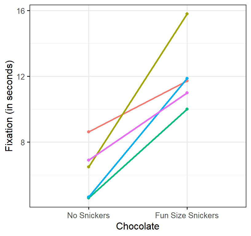
Plot of Simulation
- Spaghetti plot per person
- Each line represents a persons score from lecture 1 (no Chocolate) to lecture 2 (Chocolate)
- As you can see, most do better, some do worse
The correlation matrix:
| Corr Matrix | None | Snickers |
|---|---|---|
| None | 1 | 0.21 |
| Snickers | 0.21 | 1 |
The values are r is somewhat close to the \(\rho\) = .4, that we simulated.
Variance per cell:
| Chocolate | Varience |
|---|---|
| No Snickers | 2.849629 |
| Fun Size Snickers | 4.867386 |
Variances are not really homogeneous, but we do have an N of 5.
Conduct paired t-test in R
We use the t.test function with the argument
paired=TRUE. (Make sure the data are sorted in order of ID
number when you read the data into R). The \(df\) = the # number of subjects - 1.
T1<-t.test(Fixation~Chocolate, paired=TRUE,
           data = DataSim1)
T1
##
## Paired t-test
##
## data: Fixation by Chocolate
## t = -5.2452, df = 4, p-value = 0.006318
## alternative hypothesis: true mean difference is not equal to 0
## 95 percent confidence interval:
## -8.915821 -2.743944
## sample estimates:
## mean difference
## -5.829882APA style Report
The apa package can convert our t-test result in APA
format automatically.
library(apa)
cat(apa(T1, format = "rmarkdown", print = FALSE))t(4) = -5.25, p = .006, d = -2.35
Logic of Paired t-test
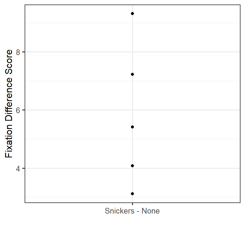
We remove the individual differences as we only care about how people Change from condition to condition. So while the raw data looks like the spaghetti plot above, what we are doing in the analysis is removing the individual differences. To remove their individual differences, we will take the difference score: Fun Size Snickers Condition - No Snickers Condition).
Given we now have difference scores we will just plot the dots:
One Sample t-test on difference Scores
Because we have one score per person (their difference between conditions) we can run a one-sample t-test and test if the difference scores are different from zero
\[t = \frac{M - \mu}{\sqrt{S^2/n}}\]
T2<-t.test(x=DataSim2$diff, y = NULL, mu=0)
T2
##
## One Sample t-test
##
## data: DataSim2$diff
## t = 5.2452, df = 4, p-value = 0.006318
## alternative hypothesis: true mean is not equal to 0
## 95 percent confidence interval:
## 2.743944 8.915821
## sample estimates:
## mean of x
## 5.829882Notice the results are identical to when we ran the t-test as a paired sample t-test.
Simplified Paired t-test Formula
To calculate this paired t-test by hand, we can calculate the differences scores (D), get the mean and variance (or S) of the difference scores. The results will be identical to the more complex formulas above which requires you subtract the individual differences using the Pearson correlation.
\[t = \frac{M_D - \mu_D}{\sqrt{S_D^2/n}}\]
Effect size
There is much debate on how to calculate a Cohen’s d for paired design. The simple formula is: (which looks like Cohen’s d for one sample t-test except on differences scores)
\[d = \frac{M_D}{S_D}\]
1 Repeated Factor: 3+ Level Designs (Repeated Measure ANOVA)
Does eating chocolate during the lecture increase Fixation to the lecture? We measure the Fixation based the mean fixation time student’s eyes are on the screen (in seconds per glance). We can collect multiple trials per condition (per person) and test between the means and run the RM ANOVA. DV = Mean Fixation time. IV = 3 level repeated factor: no chocolate (lecture #1), 1 fun size snickers (lecture #2), 1 king size snickers (lecture #3). We will simulate \(n\) = 5 students (measured at lectures 1-3) with simulated means of \(M_1\) = 5, \(M_2\) = 10, \(M_2\) = 3 (assume HOV: \(\sigma^2\) = 4). Also, the degree to which people’s responses condition is corrected, [set at \(\rho\) =.4].
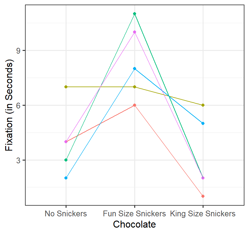
Plot of Simulation
- Spaghetti plot per person
- Each line represents a person’s score across conditions
RM ANOVA logic
In RM ANOVA we will find the variance due to the individual difference, which we can estimate by calculating the row sum, which are the sums of each subject’s scores.
One-way ANOVA Table With the formulas (conceptually simplified)
| Source | SS | DF | MS | F |
|---|---|---|---|---|
| Between | \(SS_B=nSS_{treatment}\) | \(K-1\) | \(MS_{B}=\frac{SS_B}{df_B}\) | \(\frac{MS_B}{MS_W}\) |
| Within | \(SS_W=\displaystyle \sum SS_{within}\) | \(N-K\) | \(MS_{W}=\frac{SS_W}{df_W}\) | |
| Total | \(SS_T=SS_{scores}\) | \(N-1\) |
Note: \(SS_B + SS_W = SS_T\) & \(df_B + df_W = df_T\)
One-way RM ANOVA Table With the formulas (conceptually simplified)
| Source | SS | DF | MS | F |
|---|---|---|---|---|
| \(RM_1\) | \(SS_{RM}=nSS_{all\,cell\,means}\) | \(c-1\) | \(MS_{RM}=\frac{SS_{RM}}{df_{RM}}\) | \(\frac{MS_{RM}}{MS_E}\) |
| Within | \(SS_{w}=\displaystyle \sum SS_{within}\) | |||
| \(\,Subject\,[Sub]\) | \(SS_{sub}=\frac{1}{c} SS_{subjects:\, rows\,sums}\) | \(n-1\) | \(MS_{Sub}=\frac{SS_{sub}}{df_{sub}}\) | |
| \(\,Error [Sub\,x\,RM_1]\) | \(SS_E=SS_W-SS_{sub}\) | \((n-1)(c-1)\) | \(MS_E=\frac{SS_E}{df_E}\) | |
| Total | \(SS_T=SS_{scores}\) | \(N-1\) |
Note: \(SS_{sub} + SS_E = SS_W\) & \(SS_B + SS_W = SS_T\) & \(df_B + df_W = df_T\)
Explained vs. Unexplained terms
Explained:
\(SS_{RM}\) = caused by treatment \(SS_{sub}\) = individual differences (you do not know why people are different from each other, but you can parse this variance, so we explained it).
Unexplained:
\(SS_{E}\) = This is not the individual difference; this is variance within the subjects that cannot be explained.
Assumptions
Like the paired t-test we assume HOV (\(\sigma^2_1 = \sigma^2_2 =\sigma^2_3\)), but more importantly we have assumed the correlations between the three conditions are equal (\(\rho_1 = \rho_2 = \rho_3\)). We call this compound symmetry:
\[ \mathbf{Cov} = \sigma^2\left[\begin{array} {rrrr} 1 & \rho & \rho \\ \rho & 1 & \rho \\ \rho & \rho & 1 \\ \end{array}\right] \]
When HOV is met, and we have compound symmetry, we meet the assumption of Homogeneity of covariance
Sphericity
We test for this assumption, by testing for Sphericity: Mauchly’s test of sphericity tests the variance of the difference scores between all the conditions.
\(H_0: \sigma^2_{2-1}=\sigma^2_{3-1}=\sigma^2_{3-2}\)
\(H_1: \sigma^2_{2-1}\neq\sigma^2_{3-1}\neq\sigma^2_{3-2}\)
When Sphericity is violated, we need to decrease our \(df\) to decrease the risk of type I error. We will not go into details on how this calculated, but the basic concept is that a value called \(\epsilon\) is calculated based on the degree of violation of sphericity. The more you violate this assumption, the more you correct your DF. The old school logic was to correct only when you reject the null for Mauchly’s test and conclude sphericity has been violated. The modern logic is to always correct for sphericity even if you do not reject the null of Mauchly’s test. R will follow the second approach by default.
There are two methods to calculate \(\epsilon\). The most common and marginally conservative is the Greenhouse-Geisser (GG) correction. A more powerful, but less common approach is the Huynh-Feldt (HF) correction. R defaults to GG (as do psychologists), but you can force it to report HF.
Effect sizes
SPSS & Your Book Suggests
Your book suggests an effect size which is very similar to a \(\eta^2_p\)
Remember in two-way ANOVA:
\[\eta_p^2 = \frac{SS_A}{SS_A+SS_W}\]
Since our error term is no longer \(SS_W\), now it is \(SS_E\)
\[\eta_p^2 = \frac{SS_{RM}}{SS_{RM}+SS_E}\]
R & Generalized effect size
Olejnik & Algina (2003) instead propose to use a generalized eta,
which can be compared between within & between designs (as
afex has been giving us)
\[\eta_g^2 = \frac{SS_{RM}}{SS_{RM} + SS_{sub}+ SS_E} = \frac{SS_{RM}}{SS_T} \]
You can also hand calculate (or see excel sheets) an unbiased generalized effect size
\[\omega_g^2 = \frac{df_{RM}(MS_{RM}-MS_E)}{MS_{sub}+ SS_T} \]
See Bakeman (2005) for additional issues regarding effects sizes for RM and mixed designs.
R Calculations
R Defaults
-afex calculates the RM ANOVA for us and it will
automatically correct for sphericity violations. - Error(Subject ID/RM
factor): This tells the afex that subjects vary as function RM
condition.
- It reports \(\eta_g^2\) assuming a
manipulated treatment.
library(afex)
Model.1<-aov_car(Fixation~ Chocolate + Error(SS/Chocolate),
        data = DataSim4)
Model.1
## Anova Table (Type 3 tests)
##
## Response: Fixation
## Effect df MSE F ges p.value
## 1 Chocolate 1.69, 6.77 5.36 8.65 * .611 .015
## ---
## Signif. codes: 0 '***' 0.001 '**' 0.01 '*' 0.05 '+' 0.1 ' ' 1
##
## Sphericity correction method: GGSPSS-Like report
If you want to see the results like SPSS
aov_car(Fixation~ Chocolate + Error(SS/Chocolate),
        data = DataSim4, return="univariate")
##
## Univariate Type III Repeated-Measures ANOVA Assuming Sphericity
##
## Sum Sq num Df Error SS den Df F value Pr(>F)
## (Intercept) 405.6 1 13.733 4 118.1359 0.0004067 ***
## Chocolate 78.4 2 36.267 8 8.6471 0.0100065 *
## ---
## Signif. codes: 0 '***' 0.001 '**' 0.01 '*' 0.05 '.' 0.1 ' ' 1
##
##
## Mauchly Tests for Sphericity
##
## Test statistic p-value
## Chocolate 0.81747 0.73911
##
##
## Greenhouse-Geisser and Huynh-Feldt Corrections
## for Departure from Sphericity
##
## GG eps Pr(>F[GG])
## Chocolate 0.84565 0.0155 *
## ---
## Signif. codes: 0 '***' 0.001 '**' 0.01 '*' 0.05 '.' 0.1 ' ' 1
##
## HF eps Pr(>F[HF])
## Chocolate 1.398289 0.01000649This reports the test for Mauchly’s Test (which is not significant), the uncorrected df and pvalue, but you can see the pvalues for GG and HF correction (if you applied them).
Manually Select DF Correction & \(\eta_p^2\)
You can say (HF, GG, or none)
and you can also call for \(\eta_p^2\)
with pes.
aov_car(Fixation~ Chocolate + Error(SS/Chocolate),
        data = DataSim4,
        anova_table=list(correction = "HF", es='pes'))
## Anova Table (Type 3 tests)
##
## Response: Fixation
## Effect df MSE F pes p.value
## 1 Chocolate 2, 8 4.53 8.65 * .684 .010
## ---
## Signif. codes: 0 '***' 0.001 '**' 0.01 '*' 0.05 '+' 0.1 ' ' 1
##
## Sphericity correction method: HFChallenges of Repeated Design
- Practice effects
- Carryover effects
- Order effects
- Fatigue
Solutions
- Counterbalancing
- Time between trials/distractor tasks
- Using a matched design
References
Bakeman, R. (2005). Recommended effect size statistics for repeated measures designs. Behavior research methods, 37(3), 379-384.
Olejnik, S., & Algina, J. (2003). Generalized eta and omega squared statistics: Measures of effect size for some common research designs. Psychological Methods, 8(4), 434-447. doi:10.1037/1082-989X.8.4.434