We have allowed each participant to have their own slope relative to
the sessions; meaning that each participant can respond to the therapy
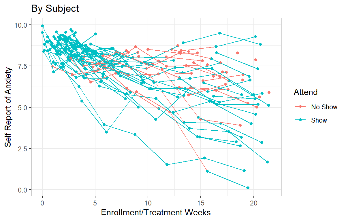
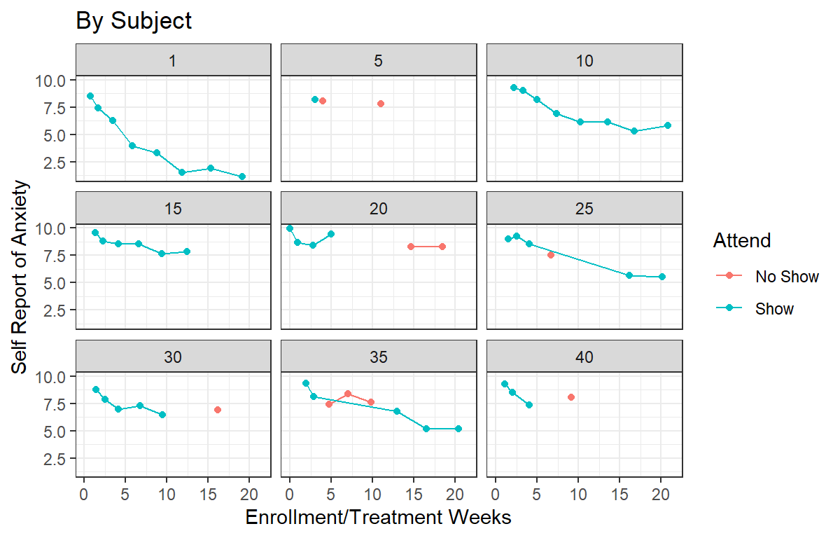
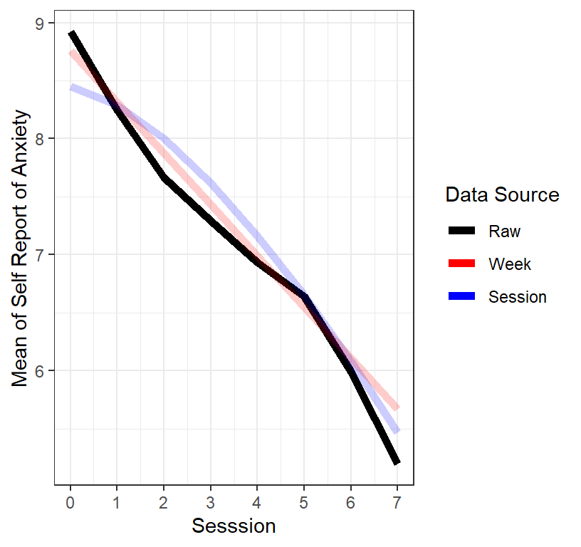
sessions in their own way. As we saw in the initial spaghetti plot, this
was probably a good idea. However, could it be that those who actually
show up to therapy sessions versus drop out might have different slopes?
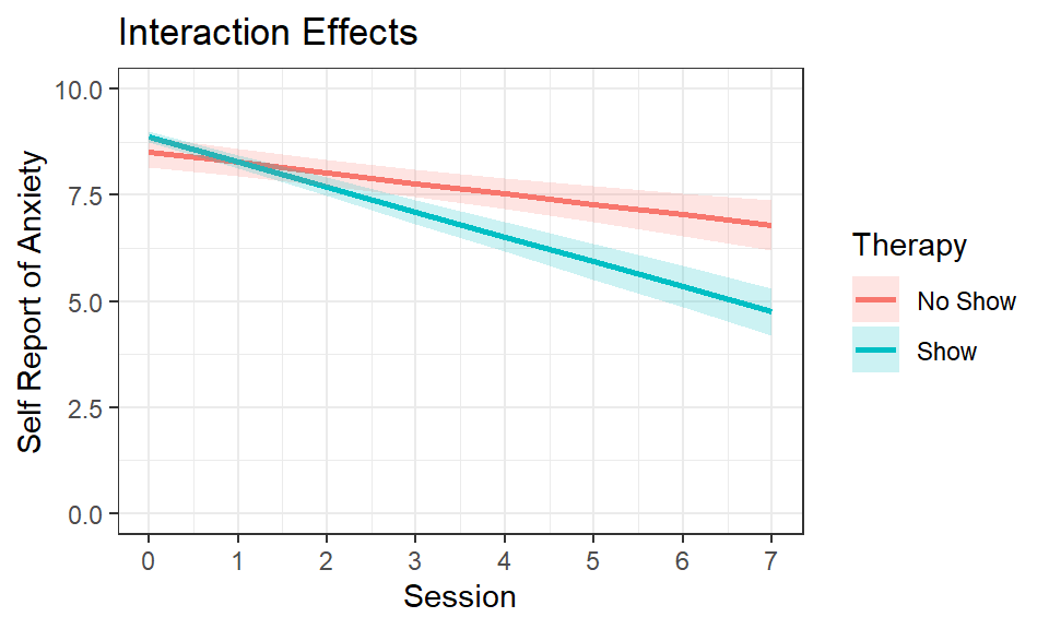
The interaction suggest there’s an overall effect, however, could it be
that there are individual slopes for each participant relative to
whether they did or did not attend therapy sessions? In other words,
should we control for whether they show up to the therapy sessions as a
random effect? The short answer is no because that is a between-subject
effect and does not vary as a function of the level 2 variable (i.e.,
the subject). The longer answer is that it depends! Case in point
below.
True Main effects?
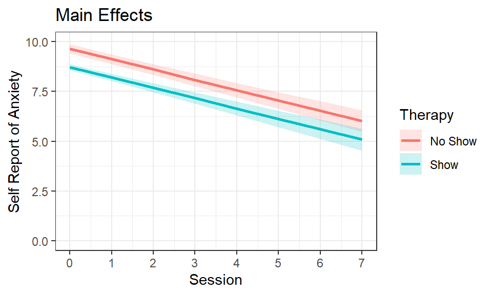
In our previous modeling, we noticed both the consistent main effect
of sessions and the simple effect of those who did were no-shows at
therapy, still showing lower self-reports of anxiety over time. From a
theoretical perspective this does not quite make sense, in that how do
people reduce their overall anxiety levels by never having gone to
therapy? If time heals all wounds then why are there therapists?
Remember, in our data all subjects started in therapy and attended at
least one or two sessions. Therefore any main effect/simple effect of
no-shows improving on anxiety could be that they learn the techniques
they needed in the first few sessions and continue to improve steadily
once they had a kickstart. Therefore an alternative method in which to
model the data may seem a little odd from a regression perspective but
makes sense in the context of this particular data set. What we’re going
to do is remove the main effect of sessions. In other words, were only
going to test the interaction between sessions and therapy attendance as
well as the main effect of therapy, given that we know people came in
and out of therapy sessions. By removing the main effect of time, we
will be creating a theoretical control group of those individuals who
never attended a therapy session, but we also want to control for
the random effect of that interaction. This allows us to remove the
main effect that is not logical (as random) and see the results we would
have expected.
Inter.Model.3<-lmer(AnxietyScore ~ Therapy+Session:Therapy+
           (1+Therapy+Session:Therapy|Subject),
         data=AxSim, REML=FALSE)
summary(Inter.Model.3 ,correlation=FALSE)
## Linear mixed model fit by maximum likelihood . t-tests use Satterthwaite's
##   method [lmerModLmerTest]
## Formula:
## AnxietyScore ~ Therapy + Session:Therapy + (1 + Therapy + Session:Therapy |
##     Subject)
##    Data: AxSim
##
##      AIC      BIC   logLik deviance df.resid
##    637.3    674.1   -308.6    617.3      282
##
## Scaled residuals:
##     Min      1Q  Median      3Q     Max
## -4.0061 -0.5087 -0.0255  0.5806  2.7752
##
## Random effects:
##  Groups   Name            Variance Std.Dev. Corr
##  Subject  (Intercept)     0.60441  0.7774
##           Therapy         0.28246  0.5315   -1.00
##           Therapy:Session 0.07572  0.2752    0.96 -0.94
##  Residual                 0.29604  0.5441
## Number of obs: 292, groups:  Subject, 45
##
## Fixed effects:
##                 Estimate Std. Error       df t value Pr(>|t|)
## (Intercept)      7.37884    0.13525 38.85585   54.56   <2e-16 ***
## Therapy          1.50092    0.12076 49.09602   12.43   <2e-16 ***
## Therapy:Session -0.59409    0.04657 47.14372  -12.76   <2e-16 ***
## ---
## Signif. codes:  0 '***' 0.001 '**' 0.01 '*' 0.05 '.' 0.1 ' ' 1
## optimizer (nloptwrap) convergence code: 0 (OK)
## boundary (singular) fit: see help('isSingular')
- Note is having some issues with our random correlations, let’s
remove them:
Inter.Model.3a<-lmer(AnxietyScore ~ Therapy+Session:Therapy+
           (1+Therapy+Session:Therapy||Subject),
         data=AxSim, REML=FALSE)
summary(Inter.Model.3a ,correlation=FALSE)
## Linear mixed model fit by maximum likelihood . t-tests use Satterthwaite's
##   method [lmerModLmerTest]
## Formula:
## AnxietyScore ~ Therapy + Session:Therapy + (1 + Therapy + Session:Therapy ||
##     Subject)
##    Data: AxSim
##
##      AIC      BIC   logLik deviance df.resid
##    676.6    702.3   -331.3    662.6      285
##
## Scaled residuals:
##     Min      1Q  Median      3Q     Max
## -4.2102 -0.4737  0.0183  0.5406  2.5074
##
## Random effects:
##  Groups    Name            Variance  Std.Dev.
##  Subject   (Intercept)     2.616e-01 5.114e-01
##  Subject.1 Therapy         3.484e-10 1.866e-05
##  Subject.2 Therapy:Session 6.798e-02 2.607e-01
##  Residual                  3.304e-01 5.748e-01
## Number of obs: 292, groups:  Subject, 45
##
## Fixed effects:
##                  Estimate Std. Error        df t value Pr(>|t|)
## (Intercept)       7.33648    0.10538  79.36444   69.62  < 2e-16 ***
## Therapy           1.51811    0.09896 253.01179   15.34  < 2e-16 ***
## Therapy:Session  -0.57147    0.04798  45.15198  -11.91 1.57e-15 ***
## ---
## Signif. codes:  0 '***' 0.001 '**' 0.01 '*' 0.05 '.' 0.1 ' ' 1
## optimizer (nloptwrap) convergence code: 0 (OK)
## boundary (singular) fit: see help('isSingular')
Plot Interaction
Results.Inter3<-Effect(c("Session","Therapy"),Inter.Model.3a,
                        xlevels=list(Session=seq(0,7,1),Therapy=c(0,1)))

Results.Inter3<-as.data.frame(Results.Inter3)
Results.Inter3$Therapy<-factor(Results.Inter3$Therapy,
                     levels=c(0,1),
                     labels=c("No Show","Show"))

Inter3.Plot <-ggplot(data = Results.Inter3,
                            aes(x = Session, y =fit))+
  geom_line(aes(color=Therapy),size=1)+
  coord_cartesian(ylim = c(0, 10))+
  geom_ribbon(aes(ymin=lower, ymax=upper,fill=Therapy),alpha=.2)+
    scale_x_continuous(breaks = seq(0, 7, by = 1)) +
  ylab("Self Report of Anxiety")+xlab("Session")+
    ggtitle("Interaction Effects") +
  theme(legend.position = "right")+theme_bw()
Inter3.Plot

Interpretation
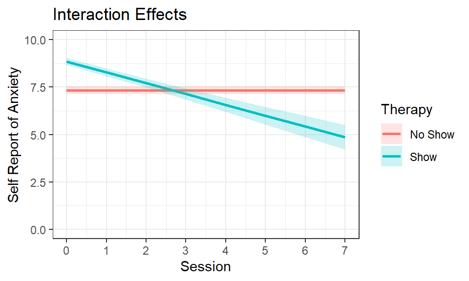
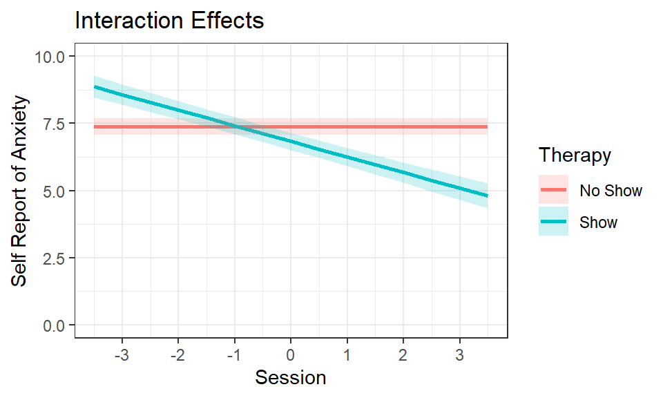
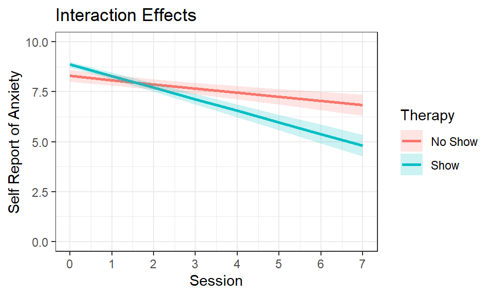
The results of this model make much more theoretical sense. Those who
never show up to therapy never improve, while those who did show up to
therapy steadily showed improvement over time. The main effect term for
therapy is necessary for interpreting the final result of the model, but
in itself is not meaningful. It is the intercept difference between the
no-show and shows conditions at session 0. In other words, as you can
clearly see the no-show group had a lower intercept than the show group.
But remember, the no-show group, in this case, is somewhat a theoretical
condition. However, the slope that we are now predicting is likely more
accurate for those individuals who actually would have attended all
therapy sessions from beginning to end.
Test Improvement?
We cannot really test the difference. First, we took away a fixed
effect and removed the random correlations and added more term. However
again remember that model fit is not always the end goal. Sometimes the
goal is to fit the data to the theory best. Model 3a is more logical
theoretically, while the interaction model (2) was just going to be a
better fit but more difficult to interpret because the data that is
fitting and interpreting is not always real. It is the goal of the
modeler to select the “best fit” and what they define as best fit is up
to them.
