Hypothesis Testing: z-tests & t-tests

Experimental Logic

The Blind Men and the Elephant

A group of blind men were traveling together, and on their trip they encounter a strange object in their path. Each blind man feels a different part of object. They then describe the object based on their partial experience. One man cries out, “it must a think branch of a tree”, say the man feeling the trunk of the elephant. “No”, says the other man, “it must be a pillar”, as he was feeling the thick leg of the elephant. The third man says, “you are both wrong, it is clearly some sort of fan”, as he feels the ear of the elephant. Of course one person must be right and the others are fools. So they beat each other up and the correct person is the one left standing! However, the elephant grows irritated with their foolishness and throws them into the river for disturbing his peace. Keep this story in mind as you try to understand the universe as you build theories to explain it with your hypotheses which are very limited in scope and biased based on your vantage point, ego, etc. - A paraphrased ancient Indian parable

Experimental Example

Step 1: I have a theory. Step 2: I have a hypothesis determined correctly from my theory. Step 3: I have a method (measurement, recruitment of the sample, & analytical tools) to test my hypothesis. Step 4: I collect some data, and it should match my prediction. When Step 4 fails, we have problems because we do not know where the failure comes from: bad theory, bad hypothesis, or bad methods (Meehl, 1978).

Theory: Behavior reinforcement of good behavior makes children happy because they know it means they have pleased adults. However, children tend to become over-excited when rewarded with objects that they know are special treats that are harmful. Cookies might be one such reward, as they know the cookie is “bad” for them but they were so good the adult broke the rules on their behalf. Unfortunately, children become overly excited by the forbidden treat, they tend to lose control and become hyperactive because they cannot yet contain their ‘id.’

Hypothesis: From this theory, we can form a hypothesis that giving children cookies will cause them to lose control of their id and become hyperactive demon children. Thus, we need to design a simple study where we give a bad reward, chocolate chip cookies. Note: No matter what we find, it does not rule out alternative theories, such as sugar (sucrose) which is the primary ingredient in cookies is digested rapidly and provides a rapid flow of sugar into the bloodstream.

Logic of Hypothesis Test

If X is true then Y is true. X is true. Therefore Y is true; However if Y is true that does not mean X is true: So, If children who eat cookies become more hyperactive than the “known” population of children (Y is true), it would be in line with our hypothesis and consistent our theory (X might be true). It does not PROVE our theory (we never knew if X was true in the first place, it was our theory/guess).

If the children do not get hyperactive (Y is false), it would not mean our theory is wrong (X could still be true). Instead, it would just mean our data does not support the hypothesis. We cannot disprove the theory; we can only provide evidence FOR it (never against it using the current methods and logic we employ). But providing evidence for the theory still not mean it was correct.

Null Hypothesis Testing using the Z-tests (Neyman & Pearson Approach)

A hypothesis test is a statistical method that uses sample data to evaluate a hypothesis about a population. Hypothesis testing is the most common type of inferential procedure. Often, we want to test how a treatment affects the population mean.

4 steps for hypothesis testing:

• State the hypothesis
• Set the Criteria Decision
• Collect Data and Compute Sample Statistics
• Make a Decision

State the hypothesis

The Null Hypothesis \(H_0\)

• States that in the general population there is no change, no difference, or no relationship
  • In an experiment, H0 predicts that the independent variable (treatment) will have no effect on the dependent variable for the population
• \(H_0\) is the hypothesis about which the final decision is to reject or fail to reject

The Scientific or Alternative Hypothesis \(H_1\)

• States that there is a change or relationship between for the general population
  • In an experiment, \(H_1\) predicts that the independent variable (treatment) will influence the dependent variable for the population.

Sample Experiment

Directional hypothesis

• \(H_0\): Chocolate chip cookies do not make children hyper
• \(H_1\): Chocolate chip cookies do make children hyper

Non-directional hypothesis

• \(H_0\): Chocolate chip cookies do not change children’s level of hyperactivity
• \(H_1\): Chocolate chip cookies do change children’s level of hyperactivity

Default in psychology is to choose the non-directional test (for reasons explained later)

Set the Criteria Decision

• Depends on the type of test, number of tests conducted, and if the hypothesis id directional or not
• Assume a normal distribution
• Let us generate a population (which we will later sample from)
• \(\mu=50, \sigma=5\)

set.seed(123)
N<-1e6
Population<-rnorm(N, mean=50,sd=5)
hist(Population,
  main="Raw Score Histogram", 
  xlab="Hyperactivity Score", ylab="Frequency")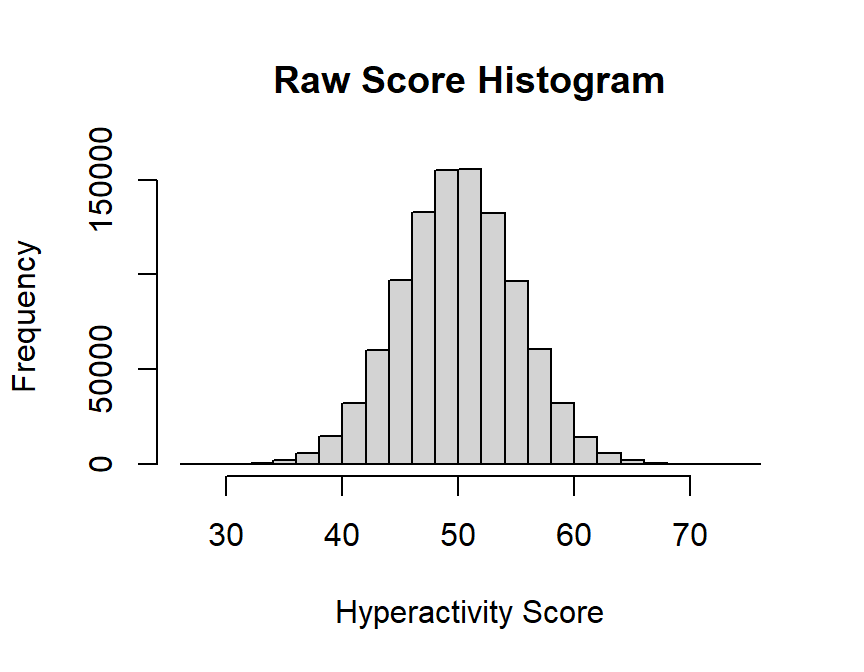

• Let us generate convert our histogram into a Probability Density Function

plot(density(scale(Population)),
  main="Probability Density Function", 
  xlab="Hyperactivity Score [z-score]", ylab="Probability", 
  xlim=c(-3.25, 3.25))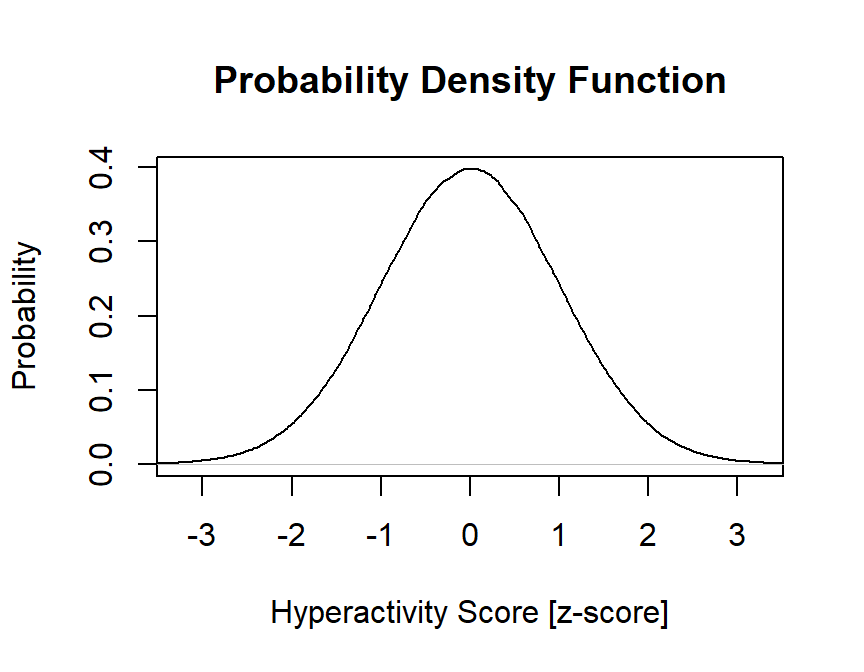

• A determination need to be made about how far sample means need to be from the population mean to reject the null.
• Problem is what could count as abnormal for this population:
• Both tails or just the lower or higher tail?
• What does the tail start and the body end?
• we set a cut-off (an Alpha level).
• common Alphas \(\alpha=.05\),\(\alpha=.01\),\(\alpha=.005\),\(\alpha=.001\),\(\alpha=.0001\)
• alpha is the degree of abnormalness (area under the curve after the cutoff)

Alpha = .05, 1-tailed

(assume abnormal is higher tail)

alpha=.05
z.cut.off=qnorm(alpha)*-1
plot(density(scale(Population)),
  main="Probability Density Function: a = .05", 
  xlab="Hyperactivity Score [z-score]", ylab="Probability", 
  xlim=c(-3.25, 3.25))
abline(v=z.cut.off, col="blue")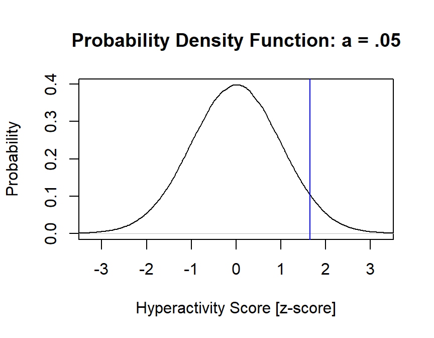

The cut off is \(z\) >1.645

Alpha = .05, 2 tailed (both sides)

Since we need to split area under the curve to both sides, \(\frac{a}{2}\)

alpha=.05/2
z.cut.lower=qnorm(alpha)
z.cut.upper=qnorm(alpha)*-1
plot(density(scale(Population)),
  main="Probability Density Function: a = .05", 
  xlab="Hyperactivity Score [z-score]", ylab="Probability", 
  xlim=c(-3.25, 3.25))
abline(v=z.cut.lower, col="blue")
abline(v=z.cut.upper, col="blue")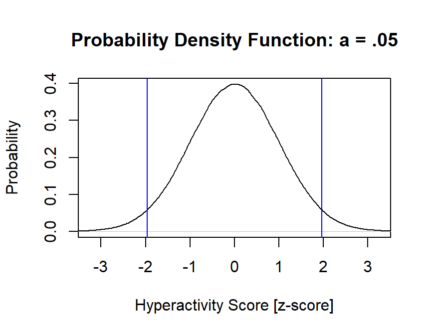

Cut offs: \(z_{lower}\) < -1.96 & \(z_{upper}\) > 1.96

• Notice they are symmetrical, this we just say \(z\) > |1.96|, two-tailed

Alpha = .05,.01,.005,.001,.0001 all 2 tailed

alphas=c(.05/2,.01/2,.005/2,.001/2,.0001/2)
z.cut.lower=qnorm(alphas)
z.cut.upper=qnorm(alphas)*-1
plot(density(scale(Population)),
  main="Probability Density Function", 
  xlab="Hyperactivity Score (Z)", ylab="Probability", 
  xlim=c(-5.25, 5.25))
abline(v=z.cut.lower, col=c("blue", "red","purple","orange","black"),lty=c(1,2,3,4,5))
abline(v=z.cut.upper, col=c("blue", "red","purple","orange","black"),lty=c(1,2,3,4,5))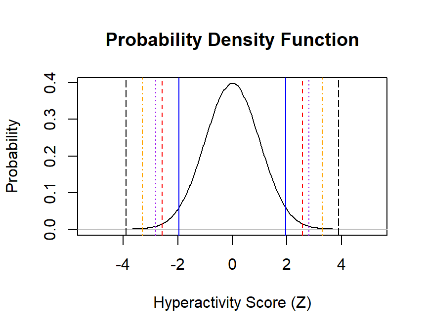

Cut offs for each alpha: - \(z_{a = .05, .01, .005, .001, .0001}\) = 1.96, 2.576, 2.807, 3.291, 3.891, two-tailed

We need to preselect an alpha (z-critical value) BEFORE conduct the experiment.

• Lets select, a = .005 (note the standard in psych tends to be .05)

Collect Data and Compute Sample Statistics

• Extract a sample of kids, \(n=36\), and feed them a bunch of cookies! (use sample function in R with replacement to select from our population)
• We will assume (as with all Z-tests) that the cookies will
• DV = We will measure their hyperactivity (which will have a random effect, but positive effect on them)

n=36
set.seed(42)
sample<-sample(Population, n, replace = TRUE)

sample.1<-sample+rnorm(n,mean=2,sd=0)
hist(sample.1,  
     main="Histogram", 
  xlab="Hyperactivity Score", ylab="Frequency")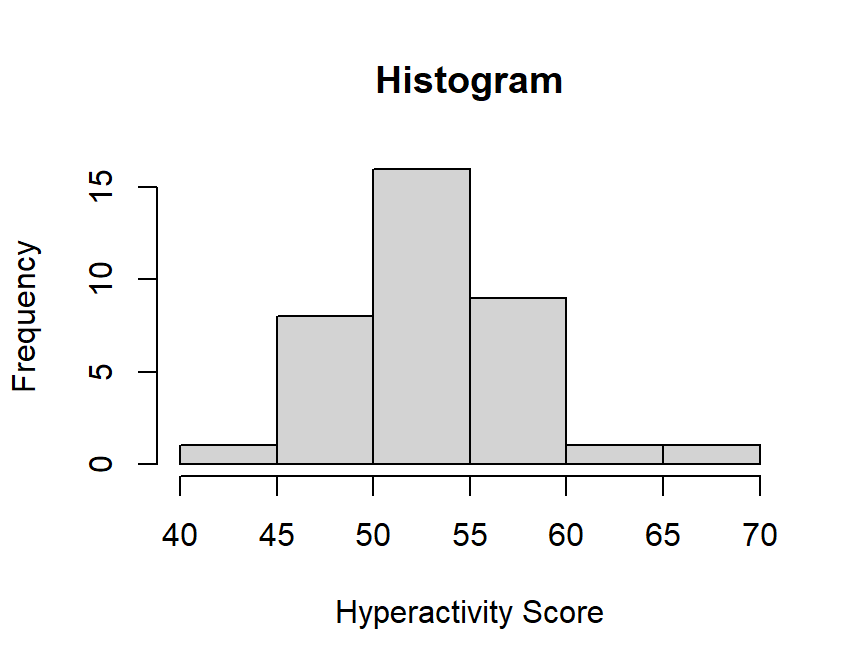

Kids on cookies showed M = 53.035 with an SD = 4.356. That is close to our population parameters! \(\mu=50, \sigma=5\), but is the sample different from the population?

Compute Sample Statistics

\[z_{test} = \frac{M - \mu}{\sigma_M}\]

where denominator is the standard error of the mean

\[\sigma_M = \frac{\sigma}{\sqrt{n}}\]

M = mean(sample.1)
Mu = 50 # given to you from the population
sigma = 5 # given to you, don't use sample SD for z-test

Ztest <- (M - Mu) / (sigma/sqrt(n))

We get a \(z_{test}\)=3.642, so is this value in the tail of the population?

Make a Decision

Two choices:

• Reject the null hypothesis - this decision can be reached when the data fall in the critical region.
  

• This means that the treatment has resulted in a likely difference between the population and the sample

• We reject the null: it is easier to prove something false than true

• Fail to reject the null: if the data do not provide strong evidence, i.e., they do not fall in the critical region, then the treatment has no effect

• Does our \(z_{test}\) fall outside the z-critical (alpha .005)?

alpha=c(.005/2)
z.cut.lower=qnorm(alpha)
z.cut.upper=qnorm(alpha)*-1
plot(density(scale(Population)),
  main="Probability Density Function: a = .005", 
  xlab="Hyperactivity Score [z-score]", ylab="Probability", 
  xlim=c(-4.25, 4.25))
abline(v=z.cut.lower, col=c("purple"),lty=c(1))
abline(v=z.cut.upper, col=c("purple"),lty=c(1))
abline(v=Ztest, col=c("red"),lty=c(2))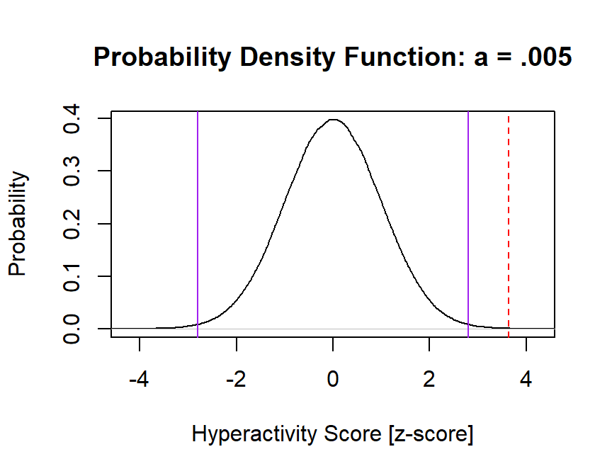

YES, our ztest > zcritical, so we REJECT the null

• We report, \(z_{test}\)=3.642 \(p < .005\) [mean \(p < a\)]
• Modern APA is report exact Pvalue

P.two.tailed=2*pnorm(-abs(Ztest))
P.one.tailed=pnorm(-abs(Ztest))

\(z_{test}\)=3.642, \(p =\) 2.7^{-4}

• But we round it (follow APA rules)

Uncertainty and Error in Hypothesis Testing

• Hypothesis testing is an inferential process because we do NOT know the actual population data and our samples could be in error
  
• When we infer we can make two (at least) types of errors (there are others).

Type I Error

• Also called false alarm or alpha error
• This occurs when a researcher rejects a null hypothesis that is actually TRUE. i.e., we reject the null even though the treatment does NOTHING
• Example, Testing zinc or ColdEase on colds using self-report as a measure of improvement
• Type 1 error, although serious, are minimized by because researchers use a stringent criterion.
• Alpha level also sets the probability of type 1 occurring.

Type II Error

• Also called miss or beta error
• Type II error occurs when a researcher fails to reject the null hypothesis that is really false.
• In other words, type II error is when the treatment has an effect and it seems like the treatment has had no effect because the hypothesis test fails to detect it
• This occurs because the sample mean is not in the critical region. The treatment worked but had a small effect.
• Example, Taking kava tea to reduce stress

Your decision	Treatment does not work (\(H_0\)=TRUE)	Treatment does work (\(H_0\)=FALSE)
Reject \(H_0\)	Type 1	Correct Decision
Retain \(H_0\)	Correct Decision	Type II

Does our alpha set the error/miss level?

• The answer is it depends. We will return this issue when we talk about statistical power

Other types of Error

• Type III and Type IV errors are not problems with procedures of the NHST, they are “user errors”. There are no singular definitions, but most are similar:

Type III error:

• Option 1: the right answer to the wrong problem (Kimball 1957, p. 134) like when hunting for ghosts - my Electromagnetic meter is beeping, that means there are ghosts here.
• Option 2: error occurs when you correctly conclude that the two groups are statistically different, but you are wrong about the direction of the difference (Very rare but can happen cause of small sampling)

Type IV error: lots of suggestions for what it should be:

• when a statistician performs the correct analysis that answers the right research questions when a simpler analysis would suffice
• asking the wrong question
• Following up an ANOVA interaction the wrong way

Factors that Influence a Hypothesis Z-Test

• Difference between the sample mean and population mean
• Sample size

Assumptions

• All statistical tests are based on assumptions.
• If you fail to meet the assumptions, then the test is compromised
• The standard deviation does not change with the treatment
• The sample must be representative of the population.

Random Sampling & Independent Observations

Two observations are independent if there is no constant, predictable relationship that occurs between the first and second variable

• In other words, each time you flip a fair coin, the probability of getting heads on each flip is the same.
• Each coin flip is independent of the preceding flip

Otherwise your data ends up like the Asch studies on social confirmatory

One-sample t-test

What do you do if you want to work with small samples and you are missing population information? This is the central problem we face in psychology.

Gosset’s First Problem

• How to use z-tests on small samples

Basic Assumption:

Gosset’s problem: \(\sigma = ?\)

\[\sigma_M = \frac{\sigma}{\sqrt{N}}\]

Gosset’s solution

\[ \sigma \approx {S}\]

Thus,

\[\sigma_M = \frac{\sigma}{\sqrt{n}} \approx S_M =\frac{S}{\sqrt{n}}\]

So the z-test,

\[z_{test} = \frac{M - \mu}{\sigma_M}\]

becomes, Student’s t-test

\[t = \frac{M - \mu}{S_M}\]

What is \(\mu\)? You would set it based on the true or hypothesized value. Often we set it at \(\mu=0\), or say in the case of IQ, \(\mu=100\). It depends on your specific question.

Gosset’s Second Problem

Can we keep assuming a normal distribution for populations to samples?

Answer: No, because we know when we sample few people are estimates are bad. So he created the t-distribution (called student’s distribution). The t-distribution is the normal distribution adjusting its shape to account for the fact in small samples you estimated the standard deviation from the sample.

x <- seq(-4, 4, length=100)
hx <- dnorm(x)

degf <- c(1, 5, 30)
colors <- c("red", "blue", "darkgreen", "black")
labels <- c("df=1", "df=5", "df=30", "normal")

plot(x, hx, type="l", lty=1, xlab="x value",
  ylab="Density", main="Comparison of t Distributions")

for (i in 1:4){
  lines(x, dt(x,degf[i]), lty=i+1, lwd=1, col=colors[i])
}

legend("topright", inset=.05, title="Distributions",
  labels, lwd=1, lty=c(2, 3, 4, 1), col=colors)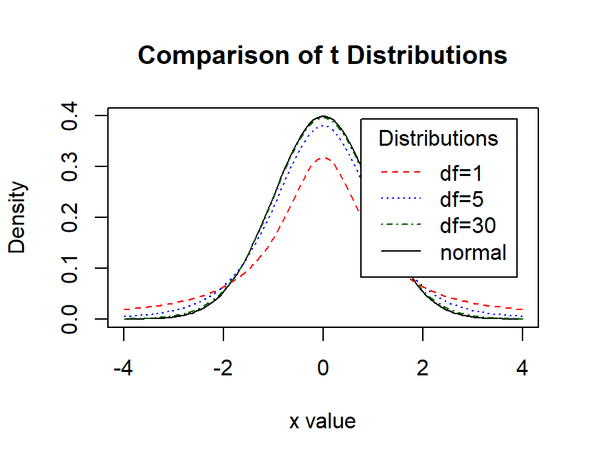

# adapted from http://www.statmethods.net/advgraphs/probability.html

• We can play with this app: https://gallery.shinyapps.io/dist_calc/

• The import thing is you need to move the boundaries changes as a function of flatness of the curve (df): you want to keep the alpha the same under the curve, this the critical regions change. So DF is needed get to tcrit.

• \(a = .05\), two-tailed. Remember [\(z = 1.96\)]

alpha = .05/2

zcrit <- -qnorm(alpha)

#create degrees of freedom
dfs <- seq(1, 30, by=1)
tcrit <- -qt(alpha,dfs)

plot(dfs, tcrit, type="l", lty=1, xlab="Degrees of Freedom",
  ylab="t-crit", main="Alpha = .05")
abline(h=zcrit, col="red")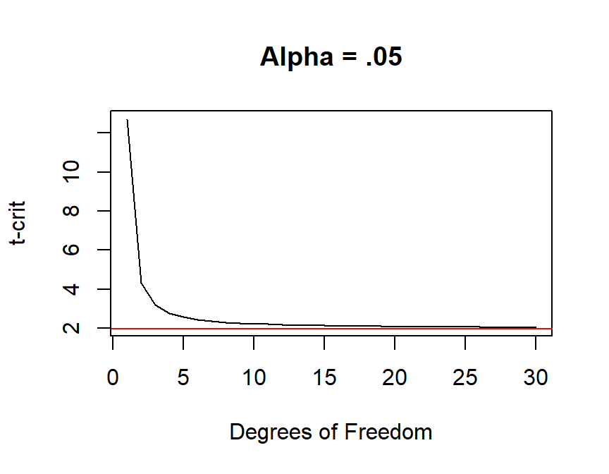

Thus \(tcrit \approx zcrit\), as \(n \Rightarrow inf\)

Confidence intervals

• What range of values can we assert we are 95% confident includes the true population parameter?
• One-sample t-test CI

\[\mu_{effect} = M \pm t_{crit}*S_M\]

\(\mu_{effect}\) would be within \(\pm\) critical tvalues and standard error of you data. The smaller your sample the larger the CI. To get 95%CI you would set your alpha to .05 to get your t-critical.

Interpret CIs

• Hot debate over what they mean (see Miller & Ulrich, 2016 vs Morey, Hoekstra, Rouder, & Wagenmakers, 2016)
• Both the word “probability” and the word “confidence” have meanings outside of their technical ones in frequentist statistics causing miss-understandings.

How to interpret CIs

• Does it actually represent the “Confidence” range which includes the population data? [as I defined it above?]
• Treat them just like NHST? [what most people do]: Interpret the interval as all the values that would not be rejected by a particular significance test.
• Follow Neyman? Avoid the problem by not interpreting CIs at all - “the confidence interval asserts nothing except that it is a sample from a confidence procedure.” [No one will accept this, but his point is well taken]
• Do Bayesian stats only? [Yeah, good luck dealing with reviewers]
• I prefer to avoid classical CIs and instead use bootstrapped CIs [we will come back to those later]

Example of one-sample t-test

• We will compare IQ (spatial reasoning) of people right after they listen to Mozart’s Sonata for Two Pianos in D Major K. 448. (Rauscher et al., 1993)

set.seed(42)
# extact a sample of 30 people, that has +9 effect on IQ
n = 30
MeanIQ.effect = 109
SDIQ = 15
Mozart.Sample <- rnorm(n,MeanIQ.effect,SDIQ)
hist(Mozart.Sample, xlab="IQ scores",main="Mozart Effect")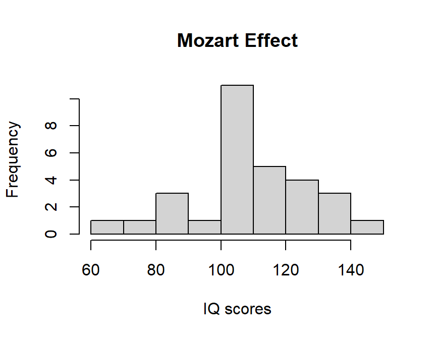

# t-test
?t.test
Mozart.t.test<-t.test(Mozart.Sample,
       alternative = c("two.sided"),
       mu = 100, paired = FALSE, var.equal = TRUE,
       conf.level = 0.95)
Mozart.t.test #call the results

## 
##  One Sample t-test
## 
## data:  Mozart.Sample
## t = 2.9179, df = 29, p-value = 0.006743
## alternative hypothesis: true mean is not equal to 100
## 95 percent confidence interval:
##  102.9993 117.0583
## sample estimates:
## mean of x 
##  110.0288

Independent Samples t-test

• what if you don’t have the population to compare to, but need to estimate their \(\mu\) via a control or comparison group?
• Independent samples t-test
• The goal of a between-subjects research study is to evaluate the mean difference between two populations (or between two treatment conditions).

\[ H_0: \mu_1 = \mu_2 \] \[ H_1: \mu_1 \neq \mu_2 \] where, \(\mu_1\) = Experimental and \(\mu_2\) = Control

Error term

• The single-sample standard error, \(S_M\) measures how much error expected between \(M\) and \(\mu\).
• The independent-samples standard error (\(S_{M1 - M2}\)) measures how much error is expected when you are using a sample mean difference (\(M1 - M2\)) to represent a population mean error.

Equal sample sizes

\[ S_{M1 - M2} = \sqrt{\frac{S^2_1}{n_1}+ \frac{S^2_2}{n_2}}\]

• Each of the two-sample means represents its own population mean, but in each case, there is some error.
  
• The amount of error associated with each sample mean can be measured by computing the standard errors.
• To calculate the total amount of error involved in using two sample means to approximate two population means, we will find the error from each sample separately and then add the two errors together.
• This formula only works when sample sizes are equal.
• When the two samples are different sizes, this formula is biased.
  
• This comes from the fact that the formula above treats the two sample variances equally. But we know that the statistics obtained from large samples are better estimates, so we need to give larger samples more weight in our estimated standard error.

Unequal sample sizes

• We are going to change the formula slightly so that we use the pooled sample variance instead of the individual sample variances. \[ S^2_p = \frac{SS_1+SS_2}{df_1+df_2}\]

• This pooled variance is going to be a weighted estimate of the variance derived from the two samples.

\[ S_{M1 - M2} = \sqrt{\frac{S^2_p}{n_1}+ \frac{S^2_p}{n_2}}\]

Formula

\[ t = \frac{M_1 - M_2 - (\mu_1 - \mu_2)} {S_{M1 - M2}}\] Where, \(\mu_1 - \mu_2 = 0\)

and \(df = (n_1 - 1) + (n_2-1)\)

Confidence Intervals for Independent Samples

\[ \mu_{effect} = (M_1-M_2) \pm t_{crit}*S_{M1 - M2}\]

Example of Independent Samples t-test

• We will compare IQ (spatial reasoning) of people right after they listen to Mozart’s Sonata for Two Pianos in D Major K. 448 to a control group who listened to Bach’s Brandenburg Concerto No. 6 in B flat major, BWV 1051 Concerto. If the effect is for Mozart only, we should not see it work when listening to Bach (matched on modality & tempo, and complexity of dueling voices)

set.seed(666)
# extact a sample of 30 people, that has +9 effect on IQ
n = 30
MozartIQ.effect = 109
SDIQ = 15
Mozart.Sample.2 <- rnorm(n,MozartIQ.effect,SDIQ)

BachIQ.effect = 110
SDIQ = 15
Bach.Sample <- rnorm(n,BachIQ.effect,SDIQ)

hist(Mozart.Sample.2, xlab="IQ scores",main="Mozart Effect",xlim = c(70,160))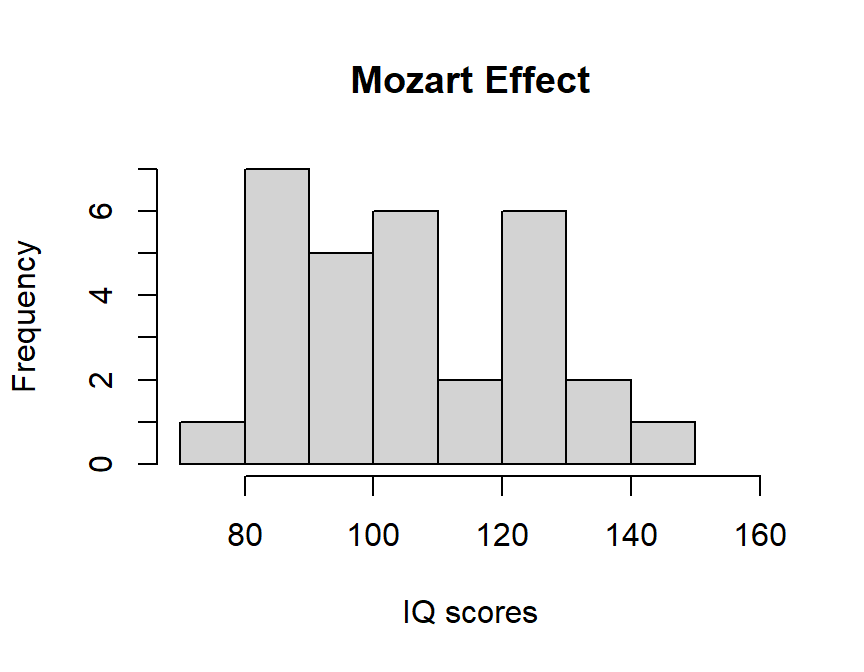

hist(Bach.Sample, xlab="IQ scores",main="Bach Effect",xlim = c(70,160))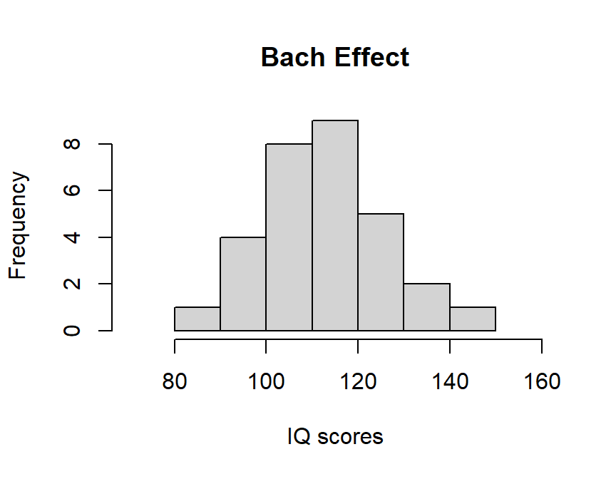

# t-test
MvsB.t.test<-t.test(x= Mozart.Sample.2, y= Bach.Sample,
       alternative = c("two.sided"),
       paired = FALSE, var.equal = TRUE,
       conf.level = 0.95)
MvsB.t.test #call the results

## 
##  Two Sample t-test
## 
## data:  Mozart.Sample.2 and Bach.Sample
## t = -1.6594, df = 58, p-value = 0.1024
## alternative hypothesis: true difference in means is not equal to 0
## 95 percent confidence interval:
##  -15.195895   1.420754
## sample estimates:
## mean of x mean of y 
##  105.1811  112.0686

So, we cannot reject the null: Bach and Mozart group had the same means (p > .05 & CIs include 0). But we cannot conclude that Mozart is not special, but maybe Bach is special too? The short answer is that Mozart was not special it was an arousal effect (Thompson et al., 2001).

Assumptions

• Observation within each sample must be independent
• The two populations from which the samples are selected must be normal
  
• The two populations from which the samples are selected must have equal variance
• Homogeneity of variance - two populations being compared must have the same variance
• We can pool our variance because it represents the same population (this satisfies homogeneity of variance)
• If your samples represent TWO DIFFERENT population you cannot pool your variance (like apples and oranges)

Testing Homogeneity of Variance

• Hartley’s F-max test or Levene’s F test
• Hartley is easy to do by hand

\[F_{max} = \frac{s^2_{larger}}{s^2_{smaller}}\] where \(df = n-1\), assumes equal samples per group, K = 2 [look up values in tables in the book]

• For Levene’s test, we need to install the car package, you would run, install.packages(‘car’) only once (until you manually update it or update R and need to reinstall it).
• This test requires we reformat the data a bit. We need to make a “data-frame”

library(car)
#Reformat
Music.Study<-data.frame(
  DV = c(Mozart.Sample.2,Bach.Sample),
  IV = c(rep("Mozart",n),rep("Bach",n))
)
# first 5 lines
head(Music.Study) 

##          DV     IV
## 1 120.29967 Mozart
## 2 139.21532 Mozart
## 3 103.67298 Mozart
## 4 139.42252 Mozart
## 5  75.74688 Mozart
## 6 120.37594 Mozart

# Lets look at boxplots quickly
boxplot(DV ~ IV, data = Music.Study)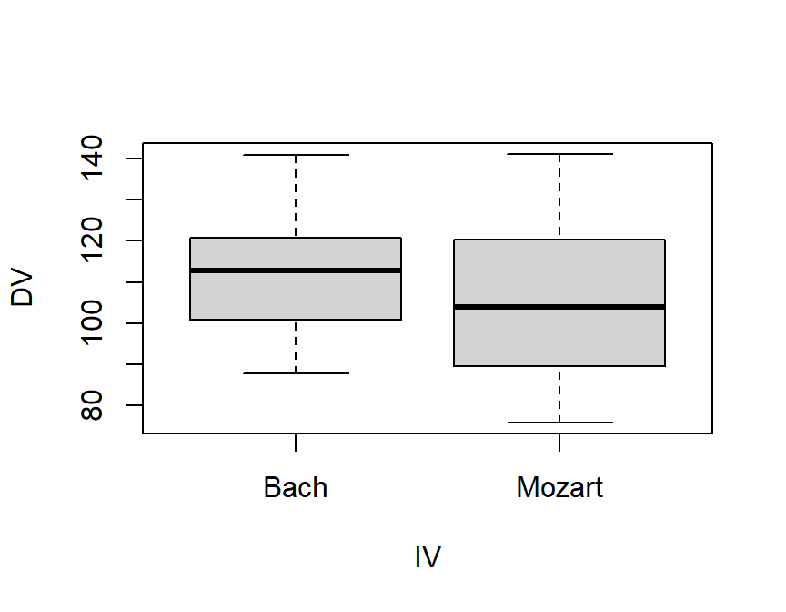

# Load functions from Car package
leveneTest(DV ~ IV, data = Music.Study)

## Levene's Test for Homogeneity of Variance (center = median)
##       Df F value  Pr(>F)  
## group  1  4.3589 0.04122 *
##       58                  
## ---
## Signif. codes:  0 '***' 0.001 '**' 0.01 '*' 0.05 '.' 0.1 ' ' 1

• Seems we have a problem. One group is more variable than the other
• We cannot fix Homogeneity of Variance (you cannot transform one group, but not the other), but we can make our test more conservative by correcting our degrees of freedom based on the degree of variances mismatch per sample size (below is an example of this type of correction)

\[df_c = \frac{(\frac{S^2_1}{n_1}+\frac{S^2_2}{n_2} )^2}{{\frac{S^2_1}{\frac{n_1}{n_1-1}}}+{\frac{S^2_2}{\frac{n_2}{n_2-1}}}}\]

Welch’s t-test (corrected for HOV)

• Note we can do our t-test on our dataframe (rather than our individual samples)
• we set var.equal=FALSE

MvsB.welch<-t.test(DV ~ IV, data = Music.Study,
       alternative = c("two.sided"),
       paired = FALSE, var.equal = FALSE,
       conf.level = 0.95)
MvsB.welch #call the results

## 
##  Welch Two Sample t-test
## 
## data:  DV by IV
## t = 1.6594, df = 52.235, p-value = 0.103
## alternative hypothesis: true difference in means between group Bach and group Mozart is not equal to 0
## 95 percent confidence interval:
##  -1.440321 15.215462
## sample estimates:
##   mean in group Bach mean in group Mozart 
##             112.0686             105.1811

• Our DF is not a smaller (and a faction)
• Not the default in R is to assume HOV problems, SPSS shows you both and lets you pick

References

Meehl, P. E. (1978). Theoretical risks and tabular asterisks: Sir Karl, Sir Ronald, and the slow progress of soft psychology. Journal of consulting and clinical Psychology, 46(4), 806.

Miller, J., & Ulrich, R. (2016). Interpreting confidence intervals: A comment on Hoekstra, Morey, Rouder, and Wagenmakers (2014). Psychonomic bulletin & review, 23(1), 124-130.

Morey, R. D., Hoekstra, R., Rouder, J. N., & Wagenmakers, E. J. (2016). Continued misinterpretation of confidence intervals: response to Miller and Ulrich. Psychonomic bulletin & review, 23(1), 131-140.

Rauscher, F. H., Shaw, G. L., & Ky, C. N. (1993). Music and spatial task performance. Nature, 365(6447), 611-611.

Thompson, W. F., Schellenberg, E. G., & Husain, G. (2001). Arousal, mood, and the Mozart effect. Psychological science, 12(3), 248-251.