Non-Linear Time & Discontinuities

Non-Linear Fit Types

Dont ask, “What is the best model for the job”. Rather, “What model is most theoretically sound.” (Singer & Willet, 2003, p.233)

• Goodness of fits & examining residuals, improvement on fits are not what always drive these approaches. You must really think about what is driving the change you see.

Major Types

• Polynomials (Power & Orthogonal) [useful generalizable approach to approximate complex growth curves]
  • You add predictors that reflect shapes (quadric = Arch/U, Cubic = S-shaped, Quartic = W/M-shaped, etc).
    • You must always have 1 data point more than the shape above a line (2 points for a line, 3 points for U, 4 points for W, etc).

Growth Curves: - Inverse Polynomials (1/Polynomials) & Hyperbola [Such as in learning theory] - Exponential (Positive & Negative Exponential, logarithmic, Power law) [seen in biological growth or perception studies] - These often can be accomplished by either transforming the DV or our measure of time - We will cover the bold ones today - Always keep in mind your cadence when you transform and remember that time can be in any unit.

Polynomials

Study Design

You have 10 participants. Five are assigned to a standard treatment of desensitization therapy, and the other five undergo a radically new type of treatment. In early sessions of desensitization therapy, clients know that they are going to be exposed to their phobia and often get anxious as their therapy time approaches. You try a radical new approach in trying to increase the degree of anxiety the experience before the actual therapy session begins. You have participants waiting outside of the door 12 minutes before the start of the therapy time, and you have a mock therapy session going on inside of the room. In the standard condition, participants do not hear what’s going into the therapy room, but they can hear voices (but not the words). In the radical condition, participants hear nothing but the voices for the first six minutes and then they hear loud yelling as a mock patient tells the therapist to keep that giant nasty spider away from them. You expect that after they hear the yelling start, they will work themselves up into anxiety frenzy just before the therapy session starts. You record from the participant a physiological measurement of anxiety once a minute which is normalized.

Before moving on to the main study, you want to make sure your manipulation worked.

Visualize Raw Data

Visualize your fit before you model is a good way to avoid problems down the line in terms of non-sensical fits: DV =Anxiety score (0 = Low to 11 High), IV = Time (0-11).

Loess Line

• Locally Weighted Scatterplot Smoothing
• Does lots of regressions on small sections of the scatter plot to get the best fit (curvy) line
• Lets you visualize complex relationships, but it can overfit the relationship (so be careful)
• Good diagnostic tool to plot what is happening on “average.” Download Data

HighAx1<-read.csv("Mixed/NonLinearTime1.csv")
HighAx1$Type<-factor(HighAx1$Treatment, 
                     levels=c(0,1),
                     labels=c("Standard", "Radical"))
HighAx1$Sound.F<-factor(HighAx1$Sound, 
                     levels=c(1,0),
                     labels=c("Screaming","Voices"))
HighAx1$Subject<-as.factor(HighAx1$Subject)

Speg<-ggplot(data = HighAx1, aes(x=Time,y=Anxiety,  color=Type))+
  geom_smooth(aes(group=Type),method='loess', se=FALSE, color='black', size=2)+
    geom_point(aes(group=Subject))+
  geom_line(aes(group=Subject))+
  ylab("Anxiety")+xlab("Time")+
  scale_y_continuous(breaks=seq(0,11,1))+
  scale_x_continuous(breaks=seq(0,11,1))+
  ggtitle("By Subject") +
  theme(legend.position = "top")+
  theme_bw()
Speg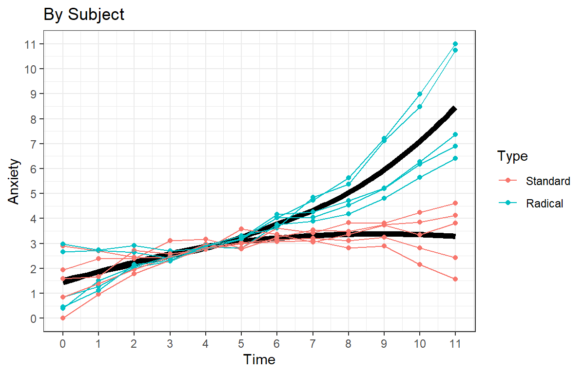

Power Polynomials

• Models that simply curves, such as quadratic or cubic effects
  
• Linear: \(Y =B_{1}X + B_0\)
• Quadratic: \(Y = B_{1}X + B_{2}X^2 + B_0\)
• Cubic: \(Y = B_{1}X + B_{2}X^2 + B_{3}X^3 + B_0\)

Visualize Subject Level

• We can add smoother per subject with each Power Polynomials (method='lm')
• This looks Linear formula=y~x or Quadratic formula=y~poly(x,2) per subject

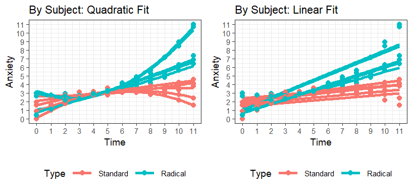
Discontinuity

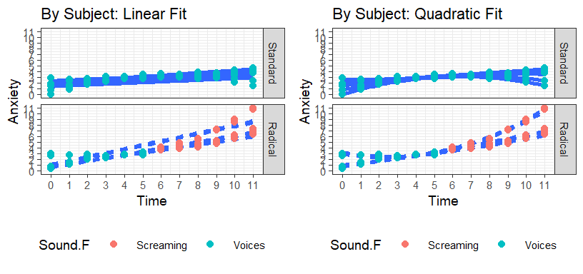
• The radical therapy does not differ from the standard therapy until 6 minutes in, so you will need to account for that, but quadratic seems to be more logical fit.

Fitting Power Polynomials

• Forward Selection Approach
  • Model 1: Linear fit
  • Model 2: Quadratic fit
  • Model i: keep going up until you are satisfied,
  • R Code you can add them manually, Anxiety + I(Anxiety^2) or with the poly command, poly(Anxiety, 2, raw=T)
• Do we want to use Type of treatment (Standard or radical) or Sound (voice whole-time vs. voice-to-screaming) [between subject condition ways of thinking about it]
• Given that standard therapy is identical to radical therapy up to 6 mins, you really want to model how the screaming changes their anxiety level, AFTER the screaming starts. We will use sound factor and not of Type therapy factor.

Linear Model Fit

• Time will not be centered (Yet)

Linear.PP<-lmer(Anxiety ~ Time*Sound.F+ (1+Time|Subject), data=HighAx1, REML=FALSE)
summary(Linear.PP, correlation=FALSE)

## Linear mixed model fit by maximum likelihood . t-tests use Satterthwaite's
##   method [lmerModLmerTest]
## Formula: Anxiety ~ Time * Sound.F + (1 + Time | Subject)
##    Data: HighAx1
## 
##      AIC      BIC   logLik deviance df.resid 
##    250.6    272.9   -117.3    234.6      112 
## 
## Scaled residuals: 
##      Min       1Q   Median       3Q      Max 
## -2.79325 -0.59057 -0.02637  0.57932  2.86639 
## 
## Random effects:
##  Groups   Name        Variance Std.Dev. Corr
##  Subject  (Intercept) 0.032526 0.18035      
##           Time        0.003536 0.05947  1.00
##  Residual             0.337005 0.58052      
## Number of obs: 120, groups:  Subject, 10
## 
## Fixed effects:
##                     Estimate Std. Error        df t value Pr(>|t|)    
## (Intercept)         -2.04852    0.54188 110.78271  -3.780 0.000254 ***
## Time                 0.90607    0.06558  99.84501  13.815  < 2e-16 ***
## Sound.FVoices        3.88930    0.54790 109.84025   7.099 1.31e-10 ***
## Time:Sound.FVoices  -0.71173    0.06924  99.35035 -10.280  < 2e-16 ***
## ---
## Signif. codes:  0 '***' 0.001 '**' 0.01 '*' 0.05 '.' 0.1 ' ' 1
## optimizer (nloptwrap) convergence code: 0 (OK)
## boundary (singular) fit: see help('isSingular')

• Note the random correlation would need to be removed

• Check the residuals of the model fit

plot(Linear.PP)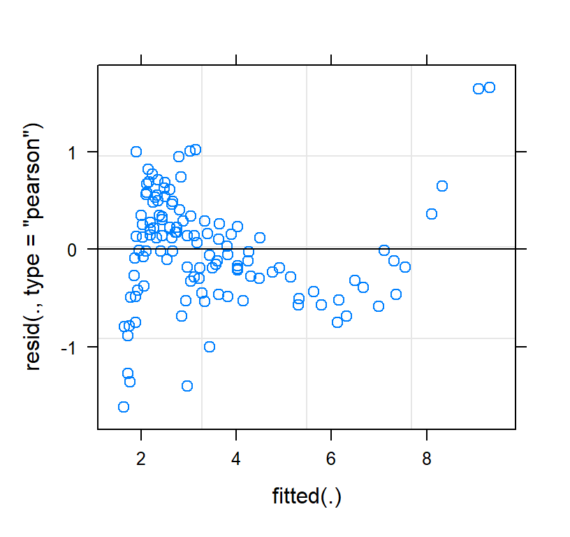

• Those are very odd. So clearly linear fit is not correct

library(effects)
Linear.PP.Fixed<-Effect(c("Time","Sound.F"),Linear.PP,
                        xlevels=list(Time=seq(0,11,1)))

Linear.PP.Fixed<-as.data.frame(Linear.PP.Fixed)

L.PP.Plot <-ggplot(data = Linear.PP.Fixed, 
                            aes(x = Time, y =fit,group=Sound.F))+
  geom_line(aes(color=Sound.F),size=2)+
  geom_ribbon(aes(ymin=lower, ymax=upper),alpha=.2)+
  ylab("Anxiety")+xlab("Time")+
  scale_y_continuous(breaks=seq(0,11,1))+
  scale_x_continuous(breaks=seq(0,11,1))+
  ggtitle("By Subject: Linear Power Poly Fit") +
  theme(legend.position = "bottom")+theme_bw()
L.PP.Plot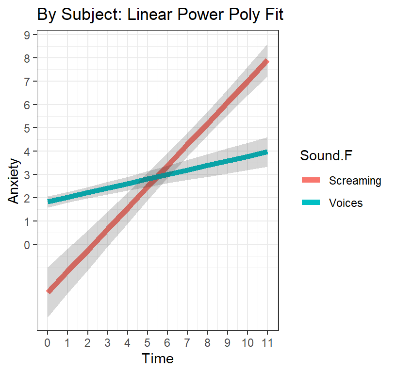

• We should not force the model to predict screaming condition BEFORE 6 minutes because that never occurs
• We can manually remove that false prediction and replot

library(dplyr)
Linear.PP.Fixed.Cleaned<-Linear.PP.Fixed %>%
  dplyr::filter(Sound.F=="Voices" | (Sound.F!="Voices" & Time>=6))

L.PP.Plot.2 <-ggplot(data = Linear.PP.Fixed.Cleaned, 
                            aes(x = Time, y =fit,group=Sound.F))+
  geom_line(aes(color=Sound.F),size=2)+
  geom_ribbon(aes(ymin=lower, ymax=upper),alpha=.2)+
  ylab("Anxiety")+xlab("Time")+
  scale_y_continuous(breaks=seq(0,11,1))+
  scale_x_continuous(breaks=seq(0,11,1))+
  ggtitle("By Subject: Linear Power Poly Fit") +
  theme(legend.position = "bottom")+theme_bw()
L.PP.Plot.2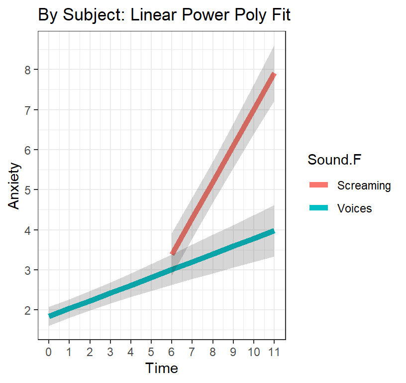

Quadratic Model Fit

• Time will not be centered (Yet)

Quad.PP<-lmer(Anxiety ~ stats::poly(Time,2,raw=TRUE)*Sound.F+ (1+stats::poly(Time,2,raw=TRUE)|Subject), data=HighAx1, REML=FALSE)
summary(Quad.PP, correlation=FALSE)

## Linear mixed model fit by maximum likelihood . t-tests use Satterthwaite's
##   method [lmerModLmerTest]
## Formula: 
## Anxiety ~ stats::poly(Time, 2, raw = TRUE) * Sound.F + (1 + stats::poly(Time,  
##     2, raw = TRUE) | Subject)
##    Data: HighAx1
## 
##      AIC      BIC   logLik deviance df.resid 
##     19.3     55.5      3.4     -6.7      107 
## 
## Scaled residuals: 
##      Min       1Q   Median       3Q      Max 
## -2.38917 -0.57582 -0.07594  0.60019  2.81510 
## 
## Random effects:
##  Groups   Name                              Variance Std.Dev. Corr       
##  Subject  (Intercept)                       0.855058 0.92469             
##           stats::poly(Time, 2, raw = TRUE)1 0.141643 0.37635  -1.00      
##           stats::poly(Time, 2, raw = TRUE)2 0.001485 0.03854   0.99 -1.00
##  Residual                                   0.031598 0.17776             
## Number of obs: 120, groups:  Subject, 10
## 
## Fixed effects:
##                                                  Estimate Std. Error        df
## (Intercept)                                       7.10066    0.96348 109.71735
## stats::poly(Time, 2, raw = TRUE)1                -1.31541    0.25254  96.39103
## stats::poly(Time, 2, raw = TRUE)2                 0.13077    0.01797  48.64731
## Sound.FVoices                                    -5.64655    0.91925  98.94311
## stats::poly(Time, 2, raw = TRUE)1:Sound.FVoices   1.76599    0.22433  99.33480
## stats::poly(Time, 2, raw = TRUE)2:Sound.FVoices  -0.15638    0.01374 102.57485
##                                                 t value Pr(>|t|)    
## (Intercept)                                       7.370 3.40e-11 ***
## stats::poly(Time, 2, raw = TRUE)1                -5.209 1.08e-06 ***
## stats::poly(Time, 2, raw = TRUE)2                 7.278 2.56e-09 ***
## Sound.FVoices                                    -6.143 1.70e-08 ***
## stats::poly(Time, 2, raw = TRUE)1:Sound.FVoices   7.872 4.42e-12 ***
## stats::poly(Time, 2, raw = TRUE)2:Sound.FVoices -11.379  < 2e-16 ***
## ---
## Signif. codes:  0 '***' 0.001 '**' 0.01 '*' 0.05 '.' 0.1 ' ' 1
## optimizer (nloptwrap) convergence code: 0 (OK)
## boundary (singular) fit: see help('isSingular')

• Note the random correlations would need to be removed

• Notice they are all significant

• Check the residuals of the model fit

plot(Quad.PP)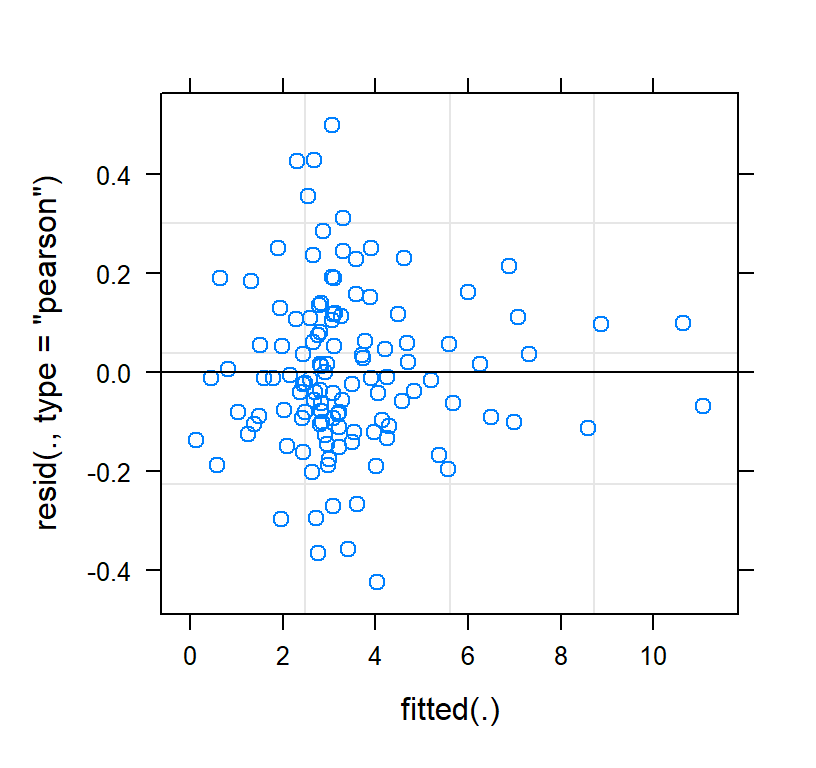

• Much better than the linear fit

Visualize Models

• Left plot = False Prediction before 6 Minutes, Right plot remove False Prediction

Quad.PP.Fixed<-Effect(c("Time","Sound.F"),Quad.PP,
                        xlevels=list(Time=seq(0,11,1)))

Quad.PP.Fixed.Cleaned<-Quad.PP.Fixed %>%
  dplyr::filter(Sound.F=="Voices" | (Sound.F!="Voices" & Time>=6))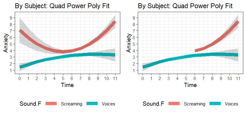

Test Improvement

• The quadratic fit is better

anova(Linear.PP,Quad.PP)

## Data: HighAx1
## Models:
## Linear.PP: Anxiety ~ Time * Sound.F + (1 + Time | Subject)
## Quad.PP: Anxiety ~ stats::poly(Time, 2, raw = TRUE) * Sound.F + (1 + stats::poly(Time, 2, raw = TRUE) | Subject)
##           npar    AIC     BIC   logLik deviance  Chisq Df Pr(>Chisq)    
## Linear.PP    8 250.59 272.895 -117.298   234.59                         
## Quad.PP     13  19.27  55.508    3.365    -6.73 241.33  5  < 2.2e-16 ***
## ---
## Signif. codes:  0 '***' 0.001 '**' 0.01 '*' 0.05 '.' 0.1 ' ' 1

Orthogonal Polynomials

• Problem with power polynomials is interpreting them independently
• The higher order terms depend on, the lower order terms
• Thus linear term can be significant cause the higher order term is significant, but there is no linear trend in the data
  • This is because power polynomials correlate with each other (they are not unique predictors)
  • For Example:

LinearTerms<-seq(0,11,1)
QuadTerms<-LinearTerms^2

• Correlation between linear and quadratic is r = 0.964. Thus they are multicollinear!
• Technically, it’s OK that they are multicollinear, but you cannot interpret each term without looking at the other (the p-values will be problematic)
• The solution to make the linear and quadratic terms correlate with each at zero (just as we did with ANOVA)
• we can use the poly code in R, but set raw = F (which is actually the default. This is also centering the data)
• Here is an example of what R is going to do:

O.Poly<-stats::poly(LinearTerms,2)

• Correlation between linear and quadratic is now r = 0. Meaning they are no longer multicollinear. Now you can see if the linear and quadratic are independently significant.

Quadratic Model Fit

• Time will not be centered (Yet)

Linear.OP<-lmer(Anxiety ~ stats::poly(Time,1)*Sound.F+ 
                  (1+stats::poly(Time,1)|Subject), data=HighAx1, REML=FALSE)

Quad.OP<-lmer(Anxiety ~ stats::poly(Time,2)*Sound.F+ 
                (1+stats::poly(Time,2)|Subject), data=HighAx1, REML=FALSE)

summary(Quad.OP, correlation=FALSE)

## Linear mixed model fit by maximum likelihood . t-tests use Satterthwaite's
##   method [lmerModLmerTest]
## Formula: Anxiety ~ stats::poly(Time, 2) * Sound.F + (1 + stats::poly(Time,  
##     2) | Subject)
##    Data: HighAx1
## 
##      AIC      BIC   logLik deviance df.resid 
##     19.1     55.3      3.4     -6.9      107 
## 
## Scaled residuals: 
##      Min       1Q   Median       3Q      Max 
## -2.40751 -0.58027 -0.07731  0.60156  2.84083 
## 
## Random effects:
##  Groups   Name                  Variance Std.Dev. Corr     
##  Subject  (Intercept)            0.27596 0.5253            
##           stats::poly(Time, 2)1  5.39867 2.3235   0.91     
##           stats::poly(Time, 2)2 23.35501 4.8327   0.99 0.85
##  Residual                        0.03103 0.1762            
## Number of obs: 120, groups:  Subject, 10
## 
## Fixed effects:
##                                     Estimate Std. Error       df t value
## (Intercept)                           5.3797     0.2959  68.0749  18.183
## stats::poly(Time, 2)1                 4.6504     3.1277 110.7452   1.487
## stats::poly(Time, 2)2                15.1064     2.1496  34.9048   7.028
## Sound.FVoices                        -2.5275     0.2547 109.3145  -9.922
## stats::poly(Time, 2)1:Sound.FVoices   1.7345     3.1431 107.5724   0.552
## stats::poly(Time, 2)2:Sound.FVoices -18.0650     1.5740 103.4921 -11.477
##                                     Pr(>|t|)    
## (Intercept)                          < 2e-16 ***
## stats::poly(Time, 2)1                  0.140    
## stats::poly(Time, 2)2               3.57e-08 ***
## Sound.FVoices                        < 2e-16 ***
## stats::poly(Time, 2)1:Sound.FVoices    0.582    
## stats::poly(Time, 2)2:Sound.FVoices  < 2e-16 ***
## ---
## Signif. codes:  0 '***' 0.001 '**' 0.01 '*' 0.05 '.' 0.1 ' ' 1
## optimizer (nloptwrap) convergence code: 0 (OK)
## boundary (singular) fit: see help('isSingular')

• Note the random correlations are probably too high and we could remove them
• Notice they are not all significant!
  • In both cases the quadradic effect is only significant. This is different from the power polynomials.
• The one problem is the estimates have lost meaning (really only the sign is meaningful)
• The effect package will read that we used poly and we can predict as normal, you will notice there is no difference in final plot. The difference is we interpret the pattern of t-values.

Quad.OP.Fixed<-Effect(c("Time","Sound.F"),Quad.OP,
                        xlevels=list(Time=seq(0,11,1)))
Quad.OP.Fixed<-as.data.frame(Quad.OP.Fixed)

Quad.OP.Fixed.Cleaned<-Quad.OP.Fixed %>%
  dplyr::filter(Sound.F=="Voices" | (Sound.F!="Voices" & Time>=6))

Q.OP.Plot <-ggplot(data = Quad.OP.Fixed.Cleaned, 
                            aes(x = Time, y =fit,group=Sound.F))+
  geom_line(aes(color=Sound.F),size=2)+
  geom_ribbon(aes(ymin=lower, ymax=upper),alpha=.2)+
  ylab("Anxiety")+xlab("Time")+
  scale_y_continuous(breaks=seq(0,11,1))+
  scale_x_continuous(breaks=seq(0,11,1))+
  ggtitle("By Subject: Quad Otho Poly Fit") +
  theme(legend.position = "bottom")+theme_bw()
Q.OP.Plot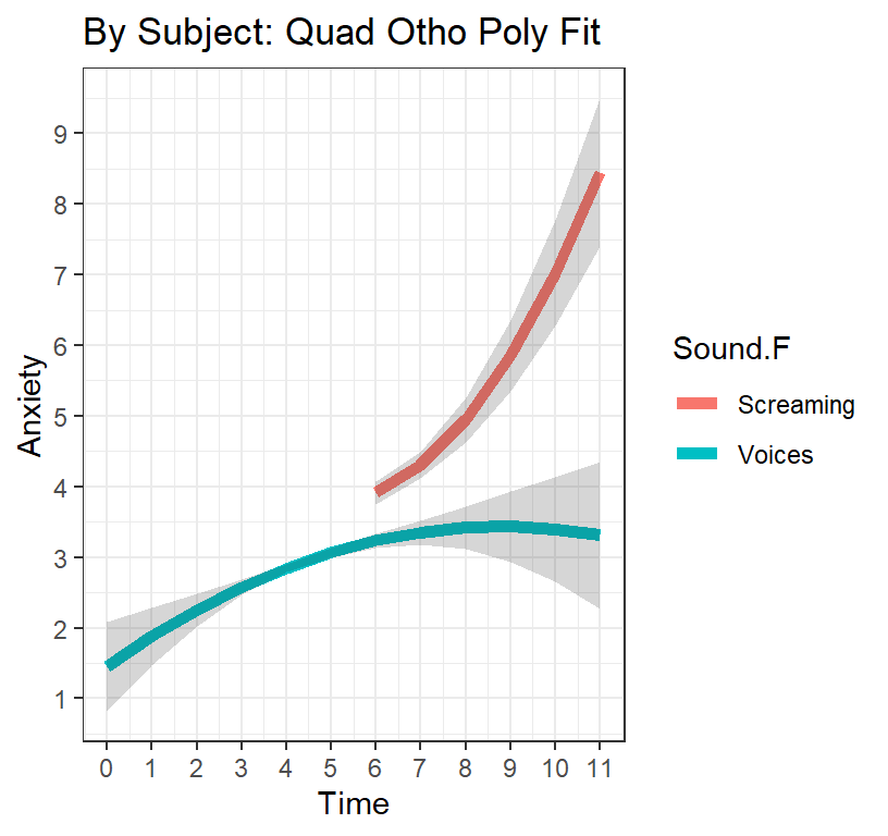

Results

The results show an overall significant positive quadratic effect on anxiety (arch-shape) for the standard treatment condition (where participants are waiting outside of the therapy room with no intervention). This suggests that as participants wait outside of the room, the increase as time goes on in the amount of anxiety feel relative to the treatment they know they’re about to undergo, but that anxiety starts to level off and even drops down a bit just before their scheduled therapy time. However, those assigned to the condition where the mock participant starts screaming at around six minutes, we see a significant discontinuity (the effect of the sound condition) where there is an immediate jump up in their anxiety level and we see a significantly negative quadratic effect (U-shape) where they get more and more anxious as their scheduled therapy time approaches. In other words, your manipulation was quite successful.

Visualizing Complete Final Model Fit

• Since this is a balanced study, we can overall model fit and the per subject fit (with dots = raw subject data)

HighAx1$QuadModelFit<-predict(Quad.OP)
Speg.Final<-ggplot()+
  geom_point(data = HighAx1, aes(x=Time,y=Anxiety, color=Sound.F))+
  geom_line(data = HighAx1, aes(x=Time,y=QuadModelFit, color=Sound.F, group=Subject))+
  geom_line(data = Quad.OP.Fixed.Cleaned, aes(x = Time, y =fit,group=Sound.F),color='blue', size=2)+
  ylab("Model Fitted Anxiety")+xlab("Time")+
  scale_y_continuous(breaks=seq(0,11,1))+
  scale_x_continuous(breaks=seq(0,11,1))+
  ggtitle("By Subject Model Fit") +
  theme(legend.position = "none")+theme_bw()
Speg.Final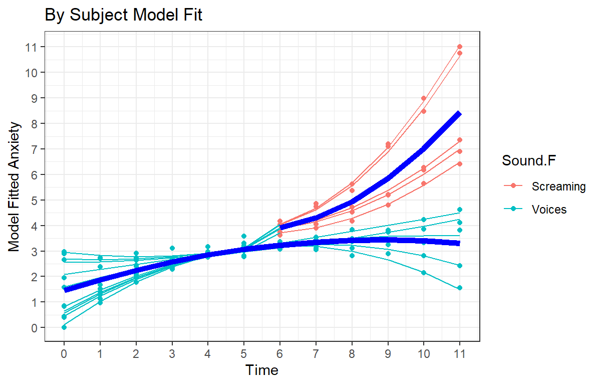

Other Types of Growth Curves

• These are models that cannot be fit with polynomials
• Logarithmic (These functions are often physical; These look more sigmoidal)
  • \(c^Y = dX\)
  • These are look more sigmoidal
• Exponential growth (like unchecked population growth)
  • \(Y = ce^{dx}\)
    • Note: Euler’s number, \(e =\) 2.7182818, is an irrational math constant and the base value of the natural log
• Power Law growth (Common function in motor control and perception experiments)
  • \(Y = cX^d\)
• In all these cases the solution is often to transform DV or Time. In power-law, you might need to transform both

Growth Curve Example

Now that you have sufficiently made half of your client’s anxiety levels go to “11” you hypothesize that given that they start out more anxious they will respond to the treatment more given that you’re putting them in the state of their maximal level of anxiety in which for you to conduct the therapy/exposure session. Thus, you expect those who came in more anxious will have the lowest levels of anxiety at the end of treatment versus those who started out with normal levels of anxiety preceding treatment. You take their Anxiety score every 3.3 mins throughout a 60-minute session

Visualize Raw Data

• DV =Anxiety score (0 = Low to 11 High)
• IV1 = Time (1-18)
• IV2 = Therapy Type (Standard or Radical)

HighAx2<-read.csv("Mixed/GrowthCurve.csv")
HighAx2$Type<-factor(HighAx2$Treatment, 
                     levels=c(0,1),
                     labels=c("Standard", "Radical"))
HighAx2$Subject<-as.factor(HighAx2$Subject)

Speg.3<-ggplot(data = HighAx2, aes(x=Time,y=Anxiety,  color=Type))+
  geom_smooth(aes(group=Type),method='loess', se=FALSE, color='black', size=2)+
    geom_point(aes(group=Subject))+
  geom_line(aes(group=Subject))+
  ylab("Anxiety")+xlab("Time")+
  scale_y_continuous(breaks=seq(0,11,1))+
  scale_x_continuous(breaks=seq(1,18,1))+
  ggtitle("By Subject") +
  theme(legend.position = "bottom")+theme_bw()
Speg.3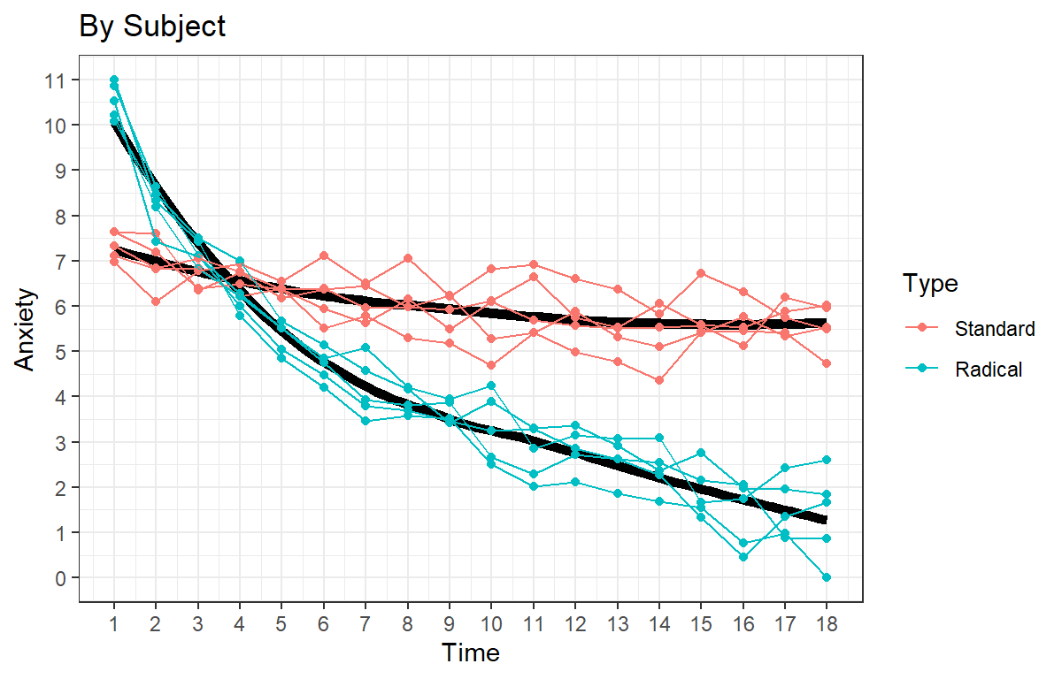

Transforms

• Polynomials might not be the best fit. Let’s try to straighten the data out as this looks somewhat exponential: Log DV | Log IV

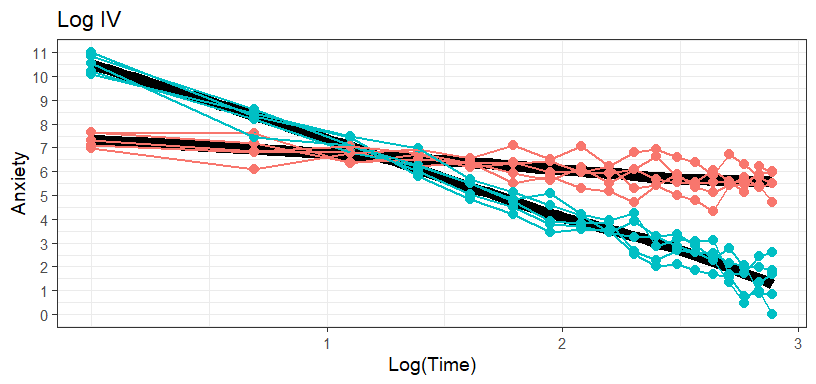
• Taking the log of the IV (Time) works best

Linear.Study2<-lmer(Anxiety ~ Time*Type+ (1+Time|Subject), data=HighAx2, REML=FALSE)
Quad.Study2<-lmer(Anxiety ~ stats::poly(Time,2)*Type+ (1+stats::poly(Time,2)|Subject), data=HighAx2, REML=FALSE)

• Check the residuals of the model fit

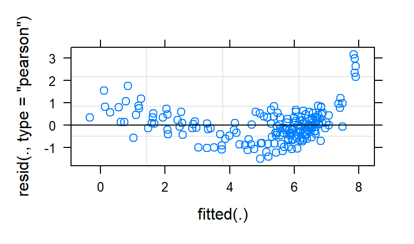
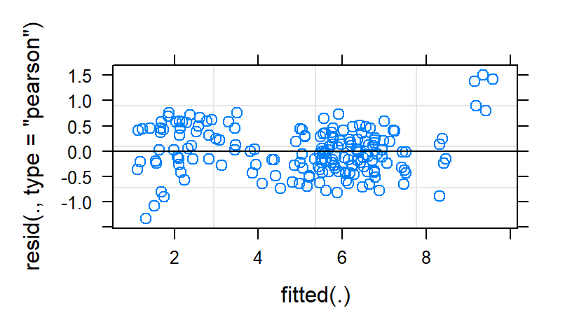
• The linear fit is terrible. The quad fit has weirdness in the tails

Log-Linear Model Fit

• Time must start at 1 [as log(0) = inf]

Linear.Log<-lmer(Anxiety ~ log(Time)*Type+ (1+log(Time)|Subject), data=HighAx2, REML=FALSE)

• Residuals look very good

plot(Linear.Log, correlation=FALSE)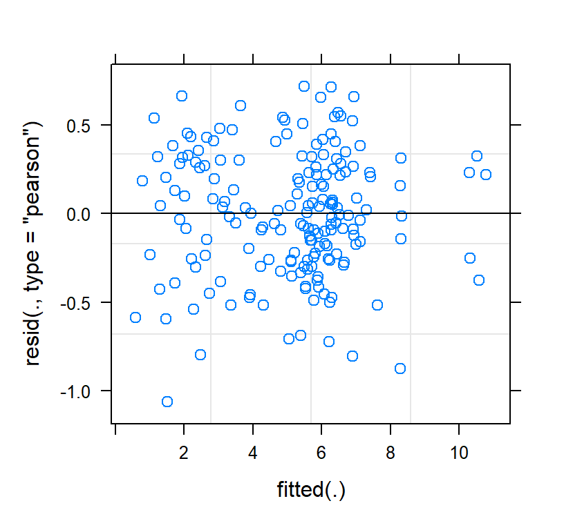

• Model Fit

summary(Linear.Log, correlation=FALSE)

## Linear mixed model fit by maximum likelihood . t-tests use Satterthwaite's
##   method [lmerModLmerTest]
## Formula: Anxiety ~ log(Time) * Type + (1 + log(Time) | Subject)
##    Data: HighAx2
## 
##      AIC      BIC   logLik deviance df.resid 
##    187.1    212.7    -85.6    171.1      172 
## 
## Scaled residuals: 
##      Min       1Q   Median       3Q      Max 
## -2.95201 -0.70486  0.00995  0.74344  1.99901 
## 
## Random effects:
##  Groups   Name        Variance Std.Dev. Corr 
##  Subject  (Intercept) 0.03067  0.1751        
##           log(Time)   0.05376  0.2319   -1.00
##  Residual             0.12920  0.3594        
## Number of obs: 180, groups:  Subject, 10
## 
## Fixed effects:
##                       Estimate Std. Error      df t value Pr(>|t|)    
## (Intercept)             7.3780     0.1313 16.0136  56.200  < 2e-16 ***
## log(Time)              -0.6472     0.1145 10.2174  -5.652 0.000196 ***
## TypeRadical             3.1273     0.1857 16.0136  16.844 1.31e-11 ***
## log(Time):TypeRadical  -2.5155     0.1620 10.2174 -15.532 1.94e-08 ***
## ---
## Signif. codes:  0 '***' 0.001 '**' 0.01 '*' 0.05 '.' 0.1 ' ' 1
## optimizer (nloptwrap) convergence code: 0 (OK)
## boundary (singular) fit: see help('isSingular')

• Notice the random correlations; they would need to be removed.

Linear.Log.Fixed<-Effect(c("Time","Type"),Linear.Log,
                        xlevels=list(Time=seq(1,18,1)))

Linear.Log.Fixed<-as.data.frame(Linear.Log.Fixed)

L.Log.Plot <-ggplot(data = Linear.Log.Fixed, 
                            aes(x = Time, y =fit,group=Type))+
  geom_line(aes(color=Type),size=2)+
  geom_ribbon(aes(ymin=lower, ymax=upper),alpha=.2)+
  ylab("Anxiety")+xlab("Time")+
  scale_y_continuous(breaks=seq(0,11,1))+
  scale_x_continuous(breaks=seq(1,18,1))+
  ggtitle("By Subject: Linear Log Fit") +
  theme(legend.position = "bottom")+theme_bw()
L.Log.Plot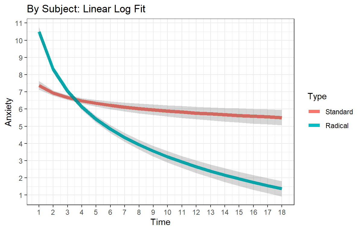

Results

While those in the standard therapy condition did show reduced anxiety by the end of the session, those in the radical therapy groups showed both significantly higher starting anxiety level than the standard group, and they showed significantly more decay in their anxiety level as indicated by the significant negative interaction.

Visualizing Complete Final Model Fit

• Plot the overall model fit and the per subject fit (with dots = raw subject data)

HighAx2$LogModelFit<-predict(Linear.Log)
Speg.Final.Study.2<-ggplot()+
  geom_point(data = HighAx2, aes(x=Time,y=Anxiety, color=Type))+
  geom_line(data = HighAx2, aes(x=Time,y=LogModelFit, color=Type, group=Subject), linetype=2)+
  geom_line(data = Linear.Log.Fixed, aes(x = Time, y =fit, color=Type,group=Type), size=2)+
  ylab("Model Fitted Anxiety")+xlab("Time")+
  scale_y_continuous(breaks=seq(0,11,1))+
  scale_x_continuous(breaks=seq(1,18,1))+
  ggtitle("By Subject Model Log Fit") +
  theme(legend.position = "none")+theme_bw()
Speg.Final.Study.2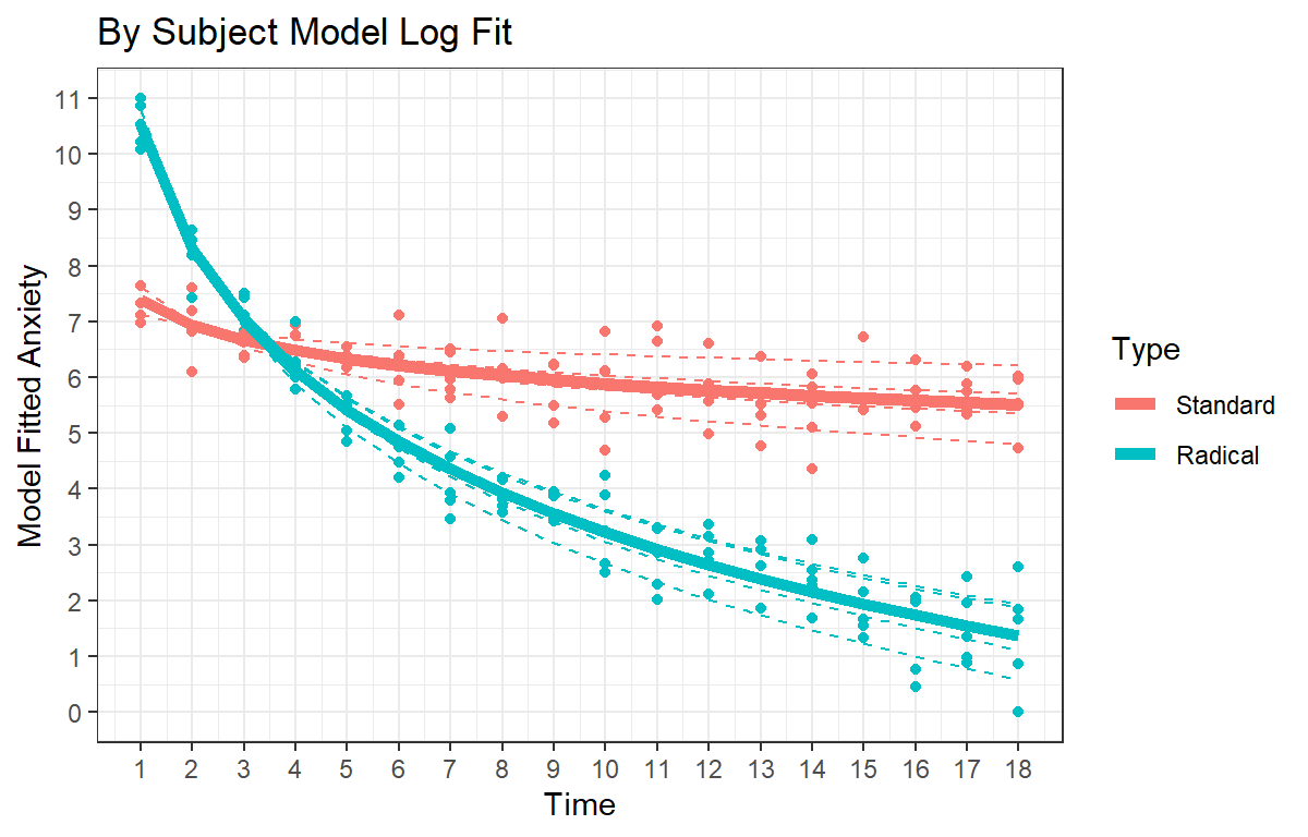

Growth Curve with a Discontinuity

You want to replicate and extend study 2 from above, but you make the treatment more radical. You know that those in the high anxiety condition (those that went to “11”) will start without more anxious and they-they will respond to the treatment more, but the might also respond to rapid onset of exposure better and you can cure them faster. Clients in both groups (standard and radical) undergo rapid exposure. You pull a lever at roughly the 35 min mark and they are dropped into a ball-pit fill with tarantulas. You expect those who in the standard group to respond poorly to their new situation, while those people in the radical group were prepared for the worst and will improve. Again, you take their Anxiety score every 3.3 mins throughout a 60-minute session.

Visualize Raw Data

• DV =Anxiety score (0 = Low to 11 High)
• IV1 = Time (1-18)
• IV2 = Therapy Type (Standard or Radical)
• IV3 =Spider pit (from Time 10-18)

HighAx3<-read.csv("Mixed/Study3.csv")
HighAx3$Type<-factor(HighAx3$Treatment, 
                     levels=c(0,1),
                     labels=c("Standard", "Radical"))
HighAx3$Location<-factor(HighAx3$Pit, 
                     levels=c(0,1),
                     labels=c("Office", "Spider Pit"))
HighAx3$Subject<-as.factor(HighAx3$Subject)

Speg.Study3<-ggplot(data = HighAx3, aes(x=Time,y=Anxiety,  color=Location))+
  facet_grid(~Type)+
  geom_smooth(aes(group=Location),method='loess', se=FALSE, color='black', size=2)+
    geom_point(aes(group=Subject))+
  geom_line(aes(group=Subject))+
  ylab("Anxiety")+xlab("Time")+
  scale_y_continuous(breaks=seq(0,11,1))+
  scale_x_continuous(breaks=seq(1,18,1))+
  ggtitle("By Subject") +
  theme(legend.position = "bottom")+theme_bw()
Speg.Study3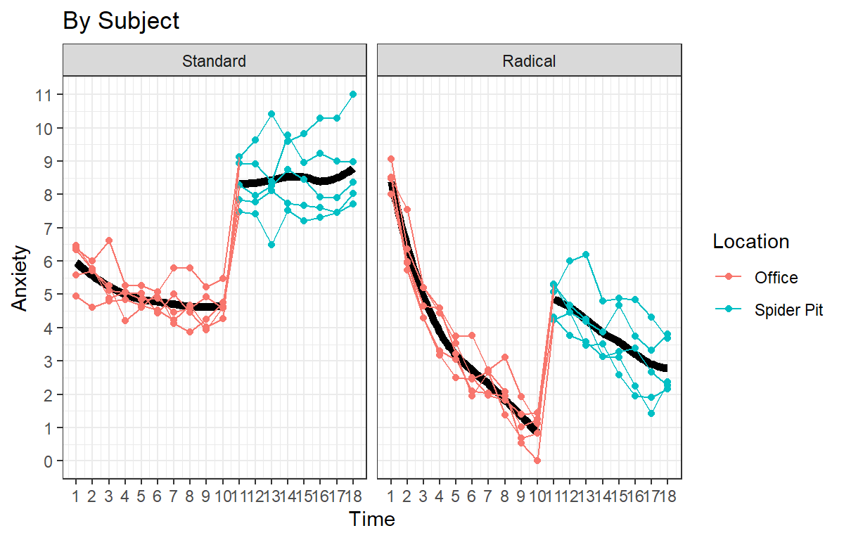

Transforms

• Like before lets log Time

Speg.Study3.log<-ggplot(data = HighAx3, aes(x=log(Time),y=Anxiety,  color=Location))+
  facet_grid(~Type)+
  geom_smooth(aes(group=Location),method='loess', se=FALSE, color='black', size=2)+
    geom_point(aes(group=Subject))+
  geom_line(aes(group=Subject))+
  ylab("Anxiety")+xlab("Time")+
  scale_y_continuous(breaks=seq(0,11,1))+
  scale_x_continuous(breaks=seq(1,18,1))+
  ggtitle("By Subject") +
  theme(legend.position = "bottom")+theme_bw()
Speg.Study3.log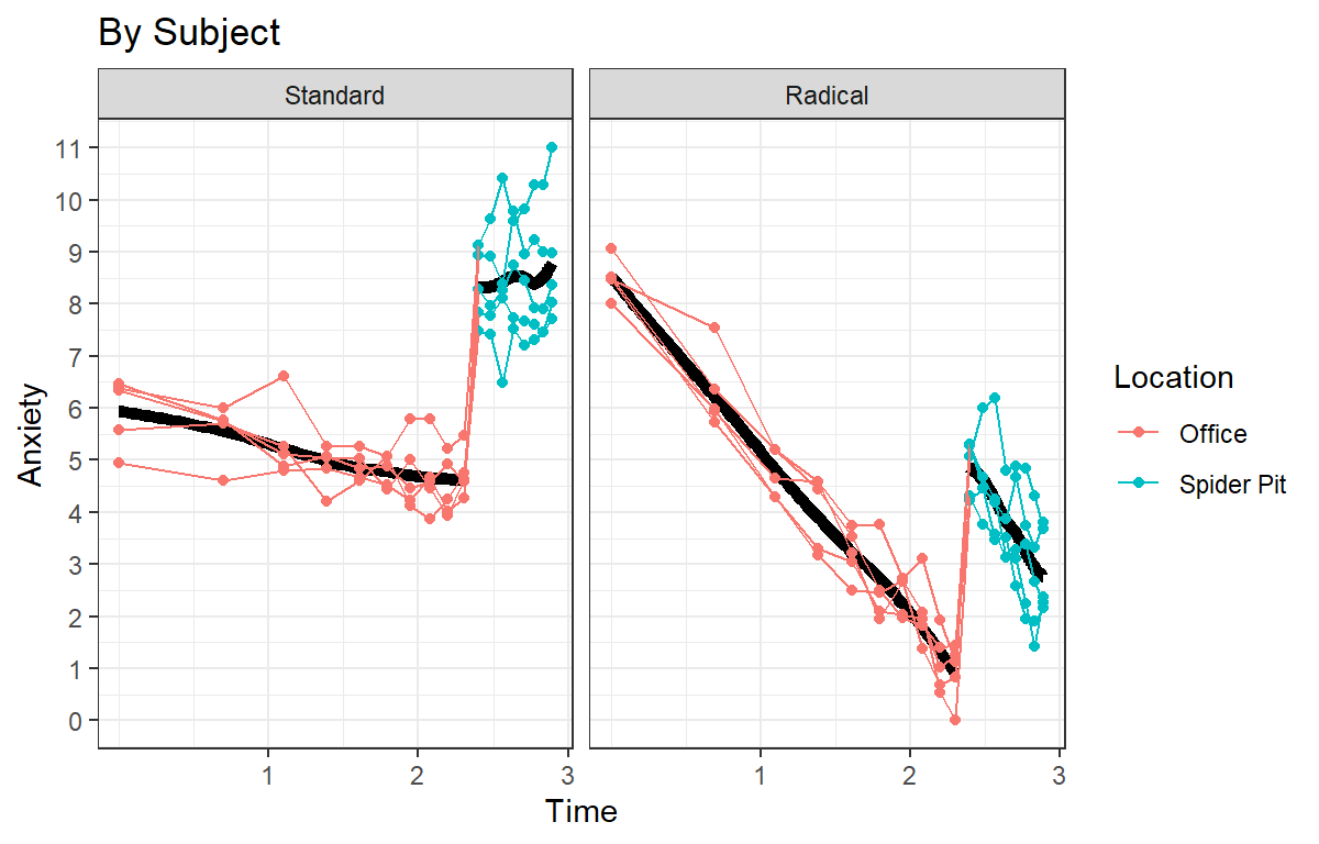

• Taking the log again makes sense

Log-Linear Model Fit with Discontinuity

• In this case Location was a within-subject variable!

Linear.Log.Study3<-lmer(Anxiety ~ log(Time)*Type*Location+ 
                          (1+log(Time)*Location|Subject), data=HighAx3, REML=FALSE)
summary(Linear.Log.Study3, correlation=FALSE)

## Linear mixed model fit by maximum likelihood . t-tests use Satterthwaite's
##   method [lmerModLmerTest]
## Formula: Anxiety ~ log(Time) * Type * Location + (1 + log(Time) * Location |  
##     Subject)
##    Data: HighAx3
## 
##      AIC      BIC   logLik deviance df.resid 
##    252.8    313.5   -107.4    214.8      161 
## 
## Scaled residuals: 
##      Min       1Q   Median       3Q      Max 
## -2.37617 -0.63871 -0.06243  0.57808  2.67636 
## 
## Random effects:
##  Groups   Name                         Variance Std.Dev. Corr             
##  Subject  (Intercept)                  0.15304  0.3912                    
##           log(Time)                    0.01339  0.1157   -0.43            
##           LocationSpider Pit           4.77592  2.1854   -0.93  0.06      
##           log(Time):LocationSpider Pit 0.86557  0.9304    0.85  0.12 -0.98
##  Residual                              0.14288  0.3780                    
## Number of obs: 180, groups:  Subject, 10
## 
## Fixed effects:
##                                          Estimate Std. Error       df t value
## (Intercept)                               5.92448    0.21667 10.65102  27.343
## log(Time)                                -0.61109    0.09267 16.65659  -6.594
## TypeRadical                               2.55865    0.30642 10.65102   8.350
## LocationSpider Pit                        0.82939    1.39768 12.92357   0.593
## log(Time):TypeRadical                    -2.63274    0.13105 16.65659 -20.089
## log(Time):LocationSpider Pit              1.25798    0.56317 12.22484   2.234
## TypeRadical:LocationSpider Pit            6.59739    1.97662 12.92357   3.338
## log(Time):TypeRadical:LocationSpider Pit -2.58070    0.79644 12.22485  -3.240
##                                          Pr(>|t|)    
## (Intercept)                              3.28e-11 ***
## log(Time)                                5.04e-06 ***
## TypeRadical                              5.36e-06 ***
## LocationSpider Pit                        0.56315    
## log(Time):TypeRadical                    4.14e-13 ***
## log(Time):LocationSpider Pit              0.04492 *  
## TypeRadical:LocationSpider Pit            0.00538 ** 
## log(Time):TypeRadical:LocationSpider Pit  0.00693 ** 
## ---
## Signif. codes:  0 '***' 0.001 '**' 0.01 '*' 0.05 '.' 0.1 ' ' 1

• We could reduce the random structure by removing the correlations or by running parsmonous approach, but we will leave this for now.

Linear.Log.Fixed.S3<-Effect(c("Time","Type","Location"),Linear.Log.Study3,
                        xlevels=list(Time=seq(1,18,1)))

Linear.Log.Fixed.S3<-as.data.frame(Linear.Log.Fixed.S3)
Linear.Log.Fixed.S3$Type<-factor(Linear.Log.Fixed.S3$Type, 
                     levels=c("Standard", "Radical"),
                     labels=c("Standard", "Radical"))

Linear.Log.Fixed.S3.Cleaned<-Linear.Log.Fixed.S3 %>%
  dplyr::filter(Location=="Office" & Time<=10| (Location!="Office" & Time>=10))


L.Log.Plot.S3 <-ggplot(data = Linear.Log.Fixed.S3.Cleaned, 
                            aes(x = Time, y =fit))+
  facet_grid(~Type)+
  geom_line(size=1, color='red')+
  geom_ribbon(aes(ymin=lower, ymax=upper),alpha=.2)+
  ylab("Anxiety")+xlab("Time")+
  scale_y_continuous(breaks=seq(0,11,1))+
  scale_x_continuous(breaks=seq(1,18,1))+
  ggtitle("By Subject: Linear Log Fit") +
  geom_vline(xintercept=10)+
  annotate("text", x = 13, y = 9, label = "Spider Pit")+
  theme(legend.position = "bottom")+theme_bw()
L.Log.Plot.S3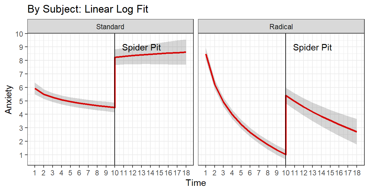

Results

In both standard and radical therapy, dropping them into the spider pit caused them to have increased anxiety, but only the those in radical therapy were able to calm down.

Notes

Always try to follow what you see and remember you are modeling at the level of the individual subject (when the subject is the level 2). These types of model are easy to over-fit (for example too many polynomials). However, underfitting can be equally as bad. Many people argue if the linear effect does not change the “story” don’t bother with the higher order. While that may be true sometimes, you can cause type II error (as the linear fit maybe weak) or even type S issues. Imagine you have a cubic effect and trying to run a line through it as the first and last data points yield the sign (but that might miss where the bulk of the data fall). Proper growth curve modeling requires careful graphing and stepwise modeling.

Generalized Additive (Mixed) Models

GAMMs are quickly becoming a new way to merge more powerful non-linear smoothing (such as using splines) to fit complex functions in the mixed model framework. They are useful for things where the shapes are rather crazy (like neuron firing). These are more bleeding edge methods and work on them is advancing quickly. Soon they will probably replace more simplistic growth curve mixed models, but as of today, they are not as flexible in the types of random structures they can handle.