Mediation

Mediation

• Baron & Kenny, 1986 (citations as of 4/13/20 =91,339)

  • See Kenny’s website for useful information: http://davidakenny.net/cm/mediate.htm

• An extremely common and popular method in social, but now used throughout psychology

• Baron & Kenny define moderator and mediator for us:

“The moderator function of third variables, which partitions a focal independent variable into subgroups that establish its domains of maximal effectiveness regarding a given dependent variable”

“The mediator function of a third variable, which represents the generative mechanism through which the focal independent variable can influence the dependent variable of interest”

• In short, the mediator explains why X->Y, and it’s through M
• Having one mediator is called simple mediation.

Simple Mediation

Preacher & Hayes, 2008 explain this figure as:

“X’s causal effect into its indirect effect on Y through M and its direct effect on Y (path c’). Path c’ a represents the effect of X on the proposed mediator, whereas path b is the effect of M on Y partialling out the effect of X. The indirect effect of X on Y through M can then be quantified as the product of a and b (i.e., ab)”

• The mediation is trying to explain the direct path seen in the total effect (the analysis without the mediation term)

Total Effect

• So we can connect the total effect back the simple moderation: \[c = c' + ab\]

\[total = direct + indirect\]

Hypothetical Example of Simple Mediation

• Children with the ability to delay gratification tend to be more successful in life (Marshmallow test)

  • You hypothesize that it is their respect/trust in of authority figures to keep their promises that is intermediating in the causal chain for success in later life

• You collect 268 4-year-olds, give them the Marshmallow test (measure their time to eat the marshmallow). Rather than waiting 20 years, you operationalize success as how they did at the end of the year on a kindergarten entrance exam. You also measure how must trust they have in authority figures (1-10 scale through an established battery for children)

• Simulation below

set.seed(42)
# For simulation of mediation steps see Hallgren, 2013
# path a strength
a=.4
# path b strength
b=.4
# path c' strength
cp=.01
# people
n <- 268
# Normal distribution of time (mins)
X <- rnorm(n, 5, 2)
# Mediator
M <- a*X+rnorm(n, 0, 1)
# Our equation to  create Y
Y <- cp*X + b*M + rnorm(n, sd=1)
#Built our data frame
Marshmallow.Data<-data.frame(Time=X,Trust=M,Success=Y)

• Graph of results

library(GGally)
library(ggplot2)
DiagPlot <- ggpairs(Marshmallow.Data,  
              lower = list(continuous = "smooth"))
DiagPlot+theme_bw()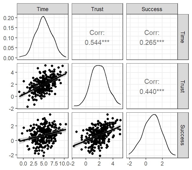

Baron and Kenny Steps to testing mediation

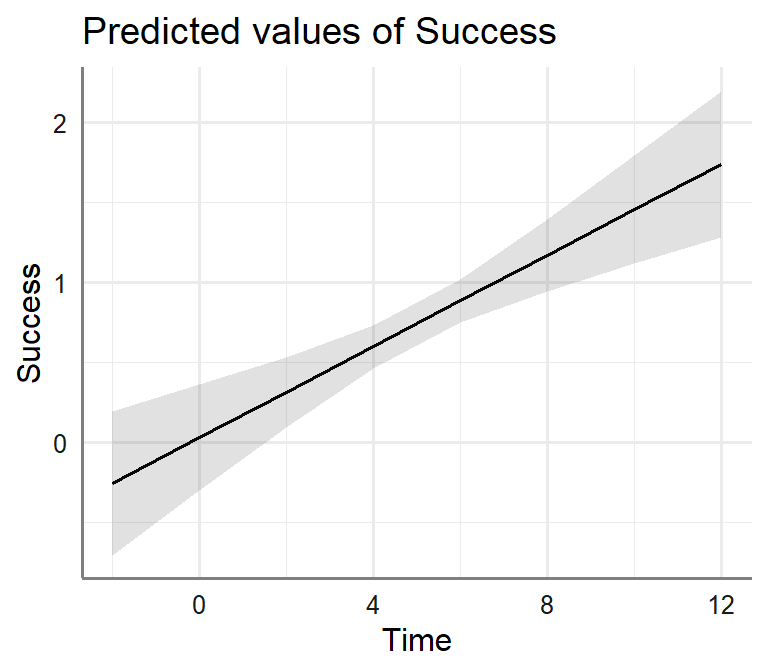
Step 1: Test Y~X

• Is there a relationship? If yes you can proceed (if not stop as you have no total effect path to try to mediate)

Model.1<-lm(Success~Time, data= Marshmallow.Data)

	Dependent variable:
	Success
Intercept	0.027 (0.169)
Time	0.143*** (0.032)
Observations	268
R2	0.070
Adjusted R2	0.067
Residual Std. Error	1.010 (df = 266)
F Statistic	20.096*** (df = 1; 266)
Note:	p<0.1; p<0.05; p<0.01

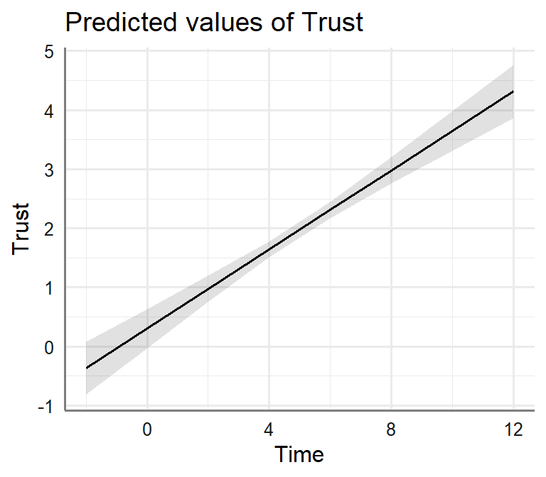
Step 2: Test M~X

• Is there a relationship? If yes you can proceed (if not stop as you have no path a)

Model.2<-lm(Trust~Time, data= Marshmallow.Data)

	Dependent variable:
	Trust
Intercept	0.305* (0.168)
Time	0.334*** (0.032)
Observations	268
R2	0.296
Adjusted R2	0.294
Residual Std. Error	1.001 (df = 266)
F Statistic	112.073*** (df = 1; 266)
Note:	p<0.1; p<0.05; p<0.01

Step 3: Test Y ~ M + X

• Is there a relationship? If yes you can proceed (if not stop as you have no path b)
• X is here as a control for M to predict X (some people say leave it out, Kenny says to leave it in)

Model.3<-lm(Success~Trust+Time, data= Marshmallow.Data)

	Dependent variable:
	Success
Intercept	-0.086 (0.159)
Trust	0.369*** (0.058)
Time	0.019 (0.035)
Observations	268
R2	0.195
Adjusted R2	0.189
Residual Std. Error	0.942 (df = 265)
F Statistic	32.059*** (df = 2; 265)
Note:	p<0.1; p<0.05; p<0.01

Step 4: Test X ~ Y + M

• Establish complete mediation
• Reverse path: M is here as a control for Y to predict X
• If there is complete mediation path c’ will go to zero
• If there is partial mediation path c’ will remain (but should get smaller) if paths a and b were meaningful

Model.4<-lm(Time~Success+Trust, data= Marshmallow.Data)

	Dependent variable:
	Time
Intercept	3.212*** (0.192)
Success	0.058 (0.106)
Trust	0.864*** (0.093)
Observations	268
R2	0.297
Adjusted R2	0.292
Residual Std. Error	1.632 (df = 265)
F Statistic	56.039*** (df = 2; 265)
Note:	p<0.1; p<0.05; p<0.01

Interpretation

• So we have complete mediation, the c’ prime path went to nearly zero
• In this case, time was not significant, but it could be with larger samples…
• The variance of time was explained by the mediator, path ab
  • but how do we test the significance of the mediator, path ab?

Significance of indirect path

• Well in our case, both path a and b were strong and significant (joint significance)
• Joint significance is an indirect test of the indirect path and is mostly holds up more modern methods (but you probably cannot publish just by showing significance on paths a and b)
• We need a direct test the significance of the indirect path (ab)
• The Baron and Kenny method was to use the Sobel’s test, which estimates the SE on terms ab of our equation, \(c = c' + ab\) and tests it against zero
• Sobel assumes of paths a and b as independent, it’s very conservative and very low powered (see http://davidakenny.net/cm/mediate.htm for details)
• There are other tests, but Sobel was the most common in its day

library(bda)
mediation.test(Marshmallow.Data$Trust,Marshmallow.Data$Time,Marshmallow.Data$Success)

##                Sobel       Aroian      Goodman
## z.value 5.478920e+00 5.461111e+00 5.496905e+00
## p.value 4.279292e-08 4.731637e-08 3.865154e-08

• Bootstrapping has replaced the Sobel’s test so we will focus on using that test in the examples
• There are two types of bootstrapping, BCa and percentile methods (remember we covered them last semester)
  • BCa can be a bit anti-conservative but more powerful, percentile method is less powerful more conservative

Mediation package in R

• You will only need Model.2 (M~X) and Model.3 (Y~M+X) from above
  • The language changes a bit in the way we talk about these things as this package can handle larger designs with control variables and many different types of regressions:
    • linear, generalized, and mixed, mixture, censored and survival
      • Note: I did 200 simulations for time, but 2000 is best if you are doing BCa.

BCa Method

library(mediation)
Med.Boot.BCa <- mediate(Model.2, Model.3, boot = TRUE, 
                        boot.ci.type = "bca", sims=200, treat="Time", mediator="Trust")
summary(Med.Boot.BCa)
plot(Med.Boot.BCa)

## 
## Causal Mediation Analysis 
## 
## Nonparametric Bootstrap Confidence Intervals with the BCa Method
## 
##                Estimate 95% CI Lower 95% CI Upper p-value    
## ACME             0.1235       0.0833         0.17  <2e-16 ***
## ADE              0.0194      -0.0413         0.08    0.53    
## Total Effect     0.1429       0.0863         0.20  <2e-16 ***
## Prop. Mediated   0.8644       0.5986         1.81  <2e-16 ***
## ---
## Signif. codes:  0 '***' 0.001 '**' 0.01 '*' 0.05 '.' 0.1 ' ' 1
## 
## Sample Size Used: 268 
## 
## 
## Simulations: 200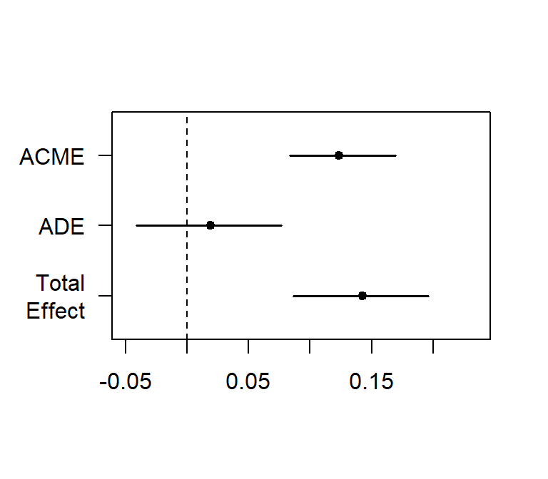

• ACME: Average Causal Mediation Effects (ACME) [total effect - direct effect]
• ADE: Average Direct Effects [total effect - indirect effect]
• Total Effect = Direct (ADE) + Indirect (ACME)
• These are unstandardized effects
• Prop. Mediated: Conceptually ACME / Total effect

Percentile Method

• By changing the code we can get percentile method over BCa

Med.Boot.perc <- mediate(Model.2, Model.3, boot = TRUE, 
                         boot.ci.type = "perc", sims=200, treat="Time", mediator="Trust")
summary(Med.Boot.perc)
plot(Med.Boot.perc)

## 
## Causal Mediation Analysis 
## 
## Nonparametric Bootstrap Confidence Intervals with the Percentile Method
## 
##                Estimate 95% CI Lower 95% CI Upper p-value    
## ACME             0.1235       0.0861         0.17  <2e-16 ***
## ADE              0.0194      -0.0387         0.08    0.54    
## Total Effect     0.1429       0.0859         0.20  <2e-16 ***
## Prop. Mediated   0.8644       0.5703         1.40  <2e-16 ***
## ---
## Signif. codes:  0 '***' 0.001 '**' 0.01 '*' 0.05 '.' 0.1 ' ' 1
## 
## Sample Size Used: 268 
## 
## 
## Simulations: 200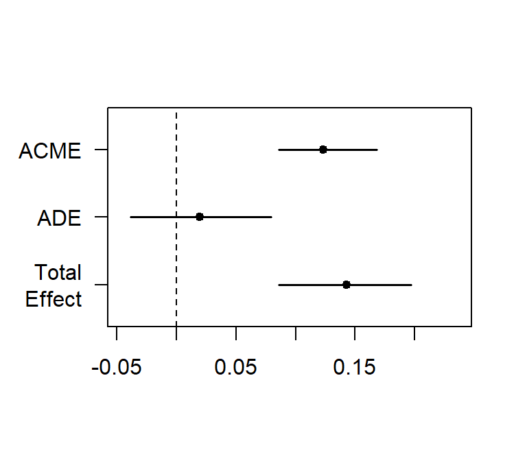

• These results match Baron and Kenny and the process macro in SPSS
• The benefit here is you test mediator in GLM or mixed (cannot be done so easily in SPSS)

Partial Mediation

• When the direct effect and indirect effect are both true
• Many times you don’t have the power for complete mediation and you might think its partial mediation
  • Kenny suggests using Hayes (2013) recommendation: never concluding that it’s complete
• Below I have created a well-powered (power = .80) examine both the direct and indirect effects

set.seed(42)
# path a strength
a=.4
# path b strength
b=.4
# path c' strength
cp=.2
# people
n <- 177
# Normal distribution of time (mins)
X <- rnorm(n, 5, 2)
# Mediator
M <- a*X+rnorm(n, 0, 1)
# Our equation to  create Y
Y <- cp*X + b*M + rnorm(n, sd=1)
#Built our data frame
Marshmallow.Data.Part<-data.frame(Time=X,Trust=M,Success=Y)

• Graph of results

DiagPlot.2 <- ggpairs(Marshmallow.Data.Part,  
              lower = list(continuous = "smooth"))
DiagPlot.2+theme_bw()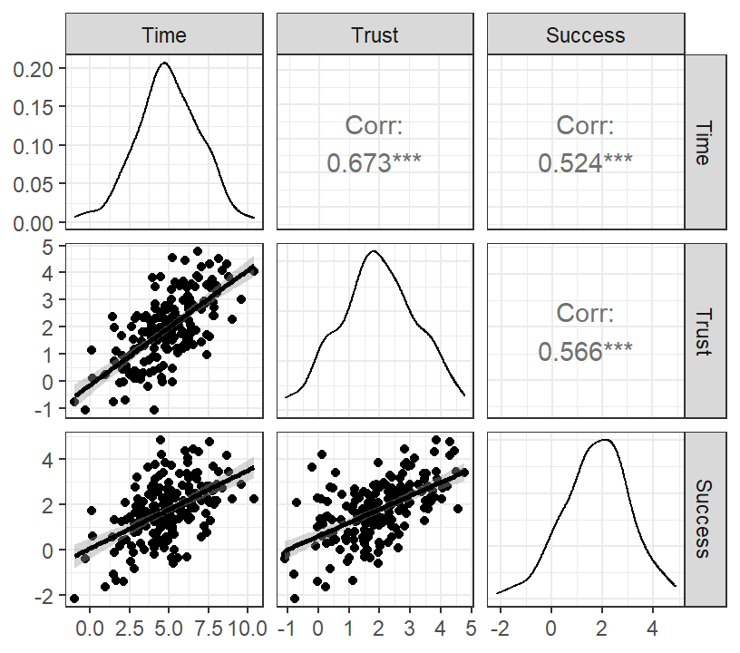

• Regression Models

Part.Model.2<-lm(Trust~Time, data= Marshmallow.Data.Part)
Part.Model.3<-lm(Success~Trust+Time, data= Marshmallow.Data.Part)

• Outcome Model

	Dependent variable:
	Success
Intercept	0.108 (0.213)
Trust	0.408*** (0.086)
Time	0.172*** (0.054)
Observations	177
R2	0.358
Adjusted R2	0.351
Residual Std. Error	1.055 (df = 174)
F Statistic	48.519*** (df = 2; 174)
Note:	p<0.1; p<0.05; p<0.01

• Mediation Analysis

Part.Med.Boot.BCa <- mediate(Part.Model.2, Part.Model.3, boot = TRUE,
                             boot.ci.type = "bca", sims=200, 
                             treat="Time", mediator="Trust")
summary(Part.Med.Boot.BCa)
plot(Part.Med.Boot.BCa,xlim=c(0,.5))

## 
## Causal Mediation Analysis 
## 
## Nonparametric Bootstrap Confidence Intervals with the BCa Method
## 
##                Estimate 95% CI Lower 95% CI Upper p-value    
## ACME             0.1726       0.0956         0.25  <2e-16 ***
## ADE              0.1724       0.0738         0.28  <2e-16 ***
## Total Effect     0.3450       0.2665         0.43  <2e-16 ***
## Prop. Mediated   0.5002       0.2644         0.75  <2e-16 ***
## ---
## Signif. codes:  0 '***' 0.001 '**' 0.01 '*' 0.05 '.' 0.1 ' ' 1
## 
## Sample Size Used: 177 
## 
## 
## Simulations: 200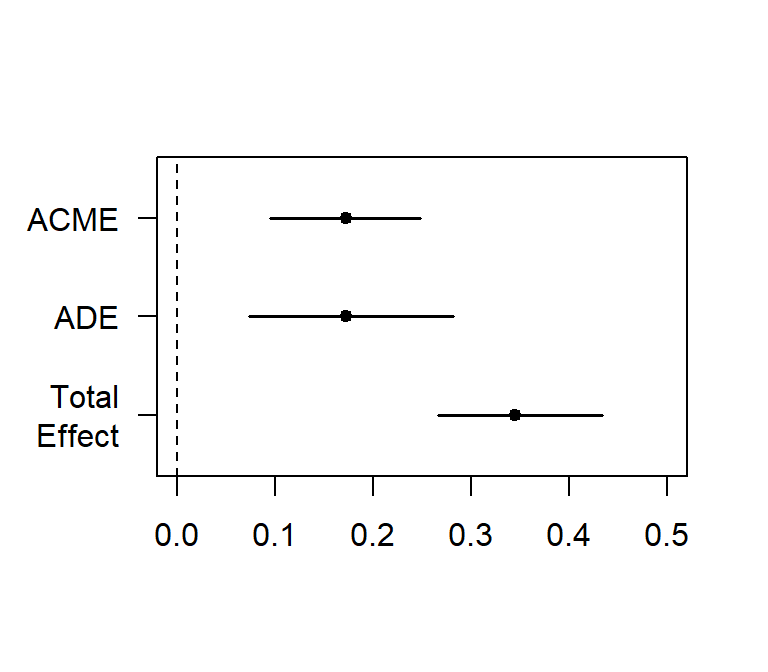

Partial Mediation with Binary Mediator

• What if your mediator is binary (GLM)? Medation package lets us test this.
• Simulation below of when the direct effect and indirect effect are both true

set.seed(42)
# path a strength
a=.5
# path b strength
b=3
# path c' strength
cp=.2
# people
n <- 1000
# Normal distribution of time (mins)
X <- rnorm(n, 5, 2)
# Mediator
z =  a*scale(X,scale=F) + rnorm(n, 0, .2)         
pr = 1/(1+exp(-z)) # pass through an inv-logit function
M = rbinom(n,1,pr)
# Our equation to  create Y
Y <- cp*X + b*M + rnorm(n, sd=1.5)
#Built our data frame
Marshmallow.Data.Bi<-data.frame(Time=X,Trust=M,Success=Y)

• Graph of results

DiagPlot.3 <- ggpairs(Marshmallow.Data.Bi,  
              lower = list(continuous = "smooth"))
DiagPlot.3+theme_bw()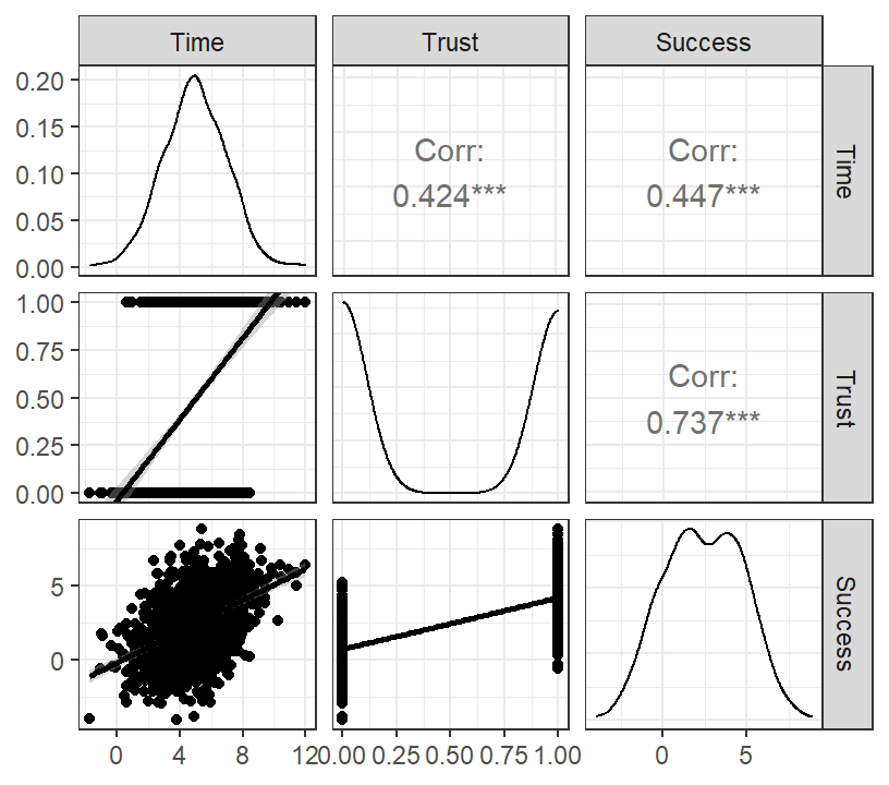

• Regression Models

Bi.Model.2<-glm(Trust~Time, data= Marshmallow.Data.Bi,
                binomial(link = "logit"))
Bi.Model.3<-lm(Success~Trust+Time, data= Marshmallow.Data.Bi)

• Plot Moderator Model

plot_model(Bi.Model.2, type = "pred", axis.lim=c(0,1),
           terms=c("Time"))+theme_sjplot2()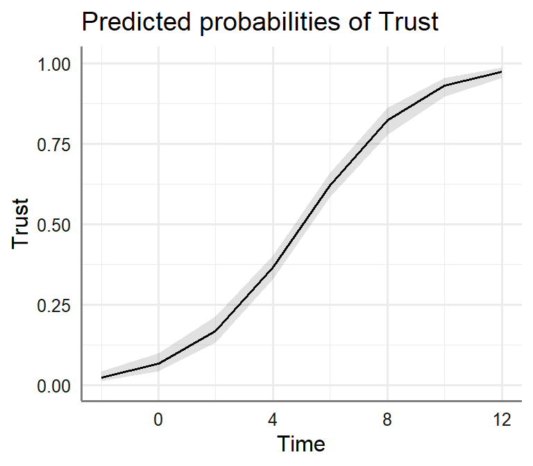

• Outcome Model

	Dependent variable:
	Success
Intercept	-0.058 (0.131)
Trust	3.127*** (0.108)
Time	0.192*** (0.027)
Observations	1,000
R2	0.565
Adjusted R2	0.564
Residual Std. Error	1.549 (df = 997)
F Statistic	646.417*** (df = 2; 997)
Note:	p<0.1; p<0.05; p<0.01

• Mediation Analysis

Bi.Med.Boot.BCa <- mediate(Bi.Model.2, Bi.Model.3, boot = TRUE,
                             boot.ci.type = "perc", sims=200, 
                             treat="Time", mediator="Trust")
summary(Bi.Med.Boot.BCa)
plot(Bi.Med.Boot.BCa,xlim=c(0,1))

## 
## Causal Mediation Analysis 
## 
## Nonparametric Bootstrap Confidence Intervals with the Percentile Method
## 
##                Estimate 95% CI Lower 95% CI Upper p-value    
## ACME             0.0969       0.0601         0.21  <2e-16 ***
## ADE              0.1919       0.1407         0.24  <2e-16 ***
## Total Effect     0.2888       0.2419         0.42  <2e-16 ***
## Prop. Mediated   0.3357       0.2241         0.54  <2e-16 ***
## ---
## Signif. codes:  0 '***' 0.001 '**' 0.01 '*' 0.05 '.' 0.1 ' ' 1
## 
## Sample Size Used: 1000 
## 
## 
## Simulations: 200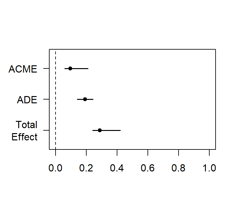

Power Analysis for Mediation

• When you plan to run mediation, you must carefully think about the power you might need.
• Because the M is collinear X you will need more subjects than you would normally think
• Kenny has worked out an easy app to estimate power for simple designs
  • https://davidakenny.shinyapps.io/MedPower/
• For larger designs, you need to build custom Monte-Carlo simulation,
  • To help simplify the Monte-Carlo simulation process you can use a shiny package built by Schoemann et al., 2017.

#library(shiny)
#runGitHub("mc_power_med", "schoam4")

• For this GUI you will need the correlations and \(SD\) between the terms
  • Here is code you can run to get that information
  • the apply function lets you calcuate \(SD\) across columns

apply(Marshmallow.Data.Part, 2, sd)
cor(Marshmallow.Data.Part)

##     Time    Trust  Success 
## 1.988666 1.250198 1.308786 
##              Time     Trust   Success
## Time    1.0000000 0.6727299 0.5242426
## Trust   0.6727299 1.0000000 0.5660804
## Success 0.5242426 0.5660804 1.0000000

Structural Equation Models [SEM] approach to Regression [Notes on SEM from Ryne Estabrook]

SEM is a unique method in that it uses visual diagrams as one way to describe a model.

• A path diagram contains all information required to specify a structural equation model.
• It contains (labeled), circles, squares, and arrows.

Path diagrams

Path diagrams are a way to present structural equation models. One uses specific shapes to represent variables and their relationships with one another.

There are two types of variables:

• Manifest variables (directly measured or observed) are represented by squares.

Other things you might see: - Triangles, which represent constants and typically are labeled “1”. - Diamonds, which deal with special functions (thresholds).

Relationships between variables are expressed as lines (paths) with one or two arrow heads.

Arrows

Two-headed arrows represent covariances or variances.

• If the heads of the arrow point to different variables, it’s a covariance.
• If both heads point to the same variable, it’s a variance (Cov(X,X)=Var(X)).

Correlation is a special type of covariance. If you want results in terms of correlations, request standardized results or make adjustment to your model.

One-headed arrows represent regressions.

• The variable pointed to is the dependent variable,
• regressed on the independent variable.

Regression in SEM

Regular regression (with a path diagram)

library(semPlot)
C.Path<-lm(Success~Time, data= Marshmallow.Data.Part)
summary(C.Path)
semPaths(C.Path, "est",
         edge.label.cex = 1,
         rotation=2,
         residuals=FALSE,
         sizeMan=10,
         color=c("blue"),
         edge.color="black",
         fade=FALSE)

## 
## Call:
## lm(formula = Success ~ Time, data = Marshmallow.Data.Part)
## 
## Residuals:
##     Min      1Q  Median      3Q     Max 
## -2.5266 -0.6639 -0.0146  0.7010  3.2600 
## 
## Coefficients:
##             Estimate Std. Error t value Pr(>|t|)    
## (Intercept)  0.05317    0.22524   0.236    0.814    
## Time         0.34502    0.04237   8.144 6.96e-14 ***
## ---
## Signif. codes:  0 '***' 0.001 '**' 0.01 '*' 0.05 '.' 0.1 ' ' 1
## 
## Residual standard error: 1.118 on 175 degrees of freedom
## Multiple R-squared:  0.2748, Adjusted R-squared:  0.2707 
## F-statistic: 66.32 on 1 and 175 DF,  p-value: 6.958e-14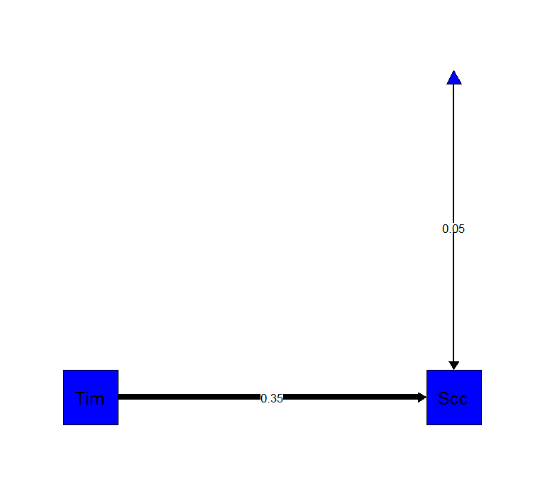

In the Laavan package (http://lavaan.ugent.be/tutorial/est.html) you write out the equations: \(Y = B_1X_1+B_0\), \(Y = Slope*X+Intercept\). I will call slope \(c\), as this would be the direct pathway in mediation. This model with fit will default to MLE (like in GLM) and we will bootstrap.

For the bootstrap there are two options:

• (se = “bootstrap”) which bootstraps to get standard errors
• (test = “bootstrap”) bootstrap based p-value

But the results should match our regression above closely. Also we can force the model to fit to fit via least squares (but we will keep it ML).

library(lavaan)
# parameters
C.lavaan <- ' # regressions
              Success ~ c*Time
              
              #Intercept
               Success ~ 1
            '

# fit model with ML
C.Fit.ML <- sem(model = C.lavaan,
            data = Marshmallow.Data.Part,
            estimator = "ML",
            se = "bootstrap",
            bootstrap = 200)

# view summary
summary(C.Fit.ML,
        fit.measures = FALSE,
        standardize = TRUE,
        rsquare = TRUE)

## lavaan 0.6-12 ended normally after 11 iterations
## 
##   Estimator                                         ML
##   Optimization method                           NLMINB
##   Number of model parameters                         3
## 
##   Number of observations                           177
## 
## Model Test User Model:
##                                                       
##   Test statistic                                 0.000
##   Degrees of freedom                                 0
## 
## Parameter Estimates:
## 
##   Standard errors                            Bootstrap
##   Number of requested bootstrap draws              200
##   Number of successful bootstrap draws             200
## 
## Regressions:
##                    Estimate  Std.Err  z-value  P(>|z|)   Std.lv  Std.all
##   Success ~                                                             
##     Time       (c)    0.345    0.041    8.407    0.000    0.345    0.524
## 
## Intercepts:
##                    Estimate  Std.Err  z-value  P(>|z|)   Std.lv  Std.all
##    .Success           0.053    0.221    0.241    0.810    0.053    0.041
## 
## Variances:
##                    Estimate  Std.Err  z-value  P(>|z|)   Std.lv  Std.all
##    .Success           1.235    0.136    9.065    0.000    1.235    0.725
## 
## R-Square:
##                    Estimate
##     Success           0.275

Plot

You can plot model estimated values.

library(semPlot)
semPaths(C.Fit.ML, "est",       
         edge.label.cex = 1,
         rotation=2,
         residuals=FALSE,
         sizeMan=10,
         color=c("blue"),
         edge.color="black",
         fade=FALSE)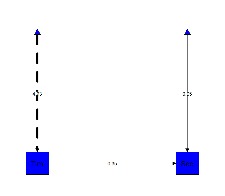

Intercept is a constant

You dont need to solve of the intercept (and we can plot standardized values)

# parameters
C.lavaan.2 <- ' # regressions
              Success ~ c*Time
            '

# fit model with ML
C.Fit.ML.2 <- sem(model = C.lavaan.2,
            data = Marshmallow.Data.Part,
            estimator = "ML",
            se = "bootstrap",
            bootstrap = 200)

# view summary
summary(C.Fit.ML.2,
        fit.measures = FALSE,
        standardize = TRUE,
        rsquare = TRUE)

## lavaan 0.6-12 ended normally after 1 iterations
## 
##   Estimator                                         ML
##   Optimization method                           NLMINB
##   Number of model parameters                         2
## 
##   Number of observations                           177
## 
## Model Test User Model:
##                                                       
##   Test statistic                                 0.000
##   Degrees of freedom                                 0
## 
## Parameter Estimates:
## 
##   Standard errors                            Bootstrap
##   Number of requested bootstrap draws              200
##   Number of successful bootstrap draws             200
## 
## Regressions:
##                    Estimate  Std.Err  z-value  P(>|z|)   Std.lv  Std.all
##   Success ~                                                             
##     Time       (c)    0.345    0.041    8.390    0.000    0.345    0.524
## 
## Variances:
##                    Estimate  Std.Err  z-value  P(>|z|)   Std.lv  Std.all
##    .Success           1.235    0.120   10.253    0.000    1.235    0.725
## 
## R-Square:
##                    Estimate
##     Success           0.275

semPaths(C.Fit.ML.2, "std", 
         edge.label.cex = 1,
         rotation=2,
         residuals=FALSE,
         sizeMan=10,
         color=c("blue"),
         edge.color="black",
         fade=FALSE)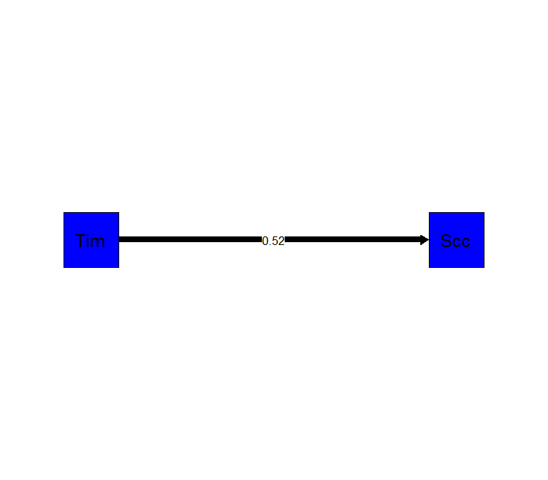

Review Mediation using Mediation package

library(mediation)
Part.Model.2<-lm(Trust~Time, data= Marshmallow.Data.Part)
Part.Model.3<-lm(Success~Trust+Time, data= Marshmallow.Data.Part)

Part.Med.Boot.BCa <- mediate(Part.Model.2, Part.Model.3, boot = TRUE,
                             boot.ci.type = "bca", sims=200, 
                             treat="Time", mediator="Trust")
summary(Part.Med.Boot.BCa)

## 
## Causal Mediation Analysis 
## 
## Nonparametric Bootstrap Confidence Intervals with the BCa Method
## 
##                Estimate 95% CI Lower 95% CI Upper p-value    
## ACME             0.1726       0.0934         0.24  <2e-16 ***
## ADE              0.1724       0.0926         0.29  <2e-16 ***
## Total Effect     0.3450       0.2645         0.42  <2e-16 ***
## Prop. Mediated   0.5002       0.2796         0.74  <2e-16 ***
## ---
## Signif. codes:  0 '***' 0.001 '**' 0.01 '*' 0.05 '.' 0.1 ' ' 1
## 
## Sample Size Used: 177 
## 
## 
## Simulations: 200

Mediation through SEM

For details on the package see here: http://lavaan.ugent.be/tutorial/syntax1.html

Note: := below assignes paramaters on the fly.

library(lavaan)

# parameters
hayes4 <- ' # direct effect
              Success ~ c*Time
              direct := c

            # regressions
              Trust ~ a*Time
              Success ~ b*Trust

            # indirect effect (a*b)
              indirect := a*b

            # total effect
              total := c + (a*b)

            # Prop
              prop := indirect/total'
 
# fit model
sem4 <- sem(model = hayes4,
            data = Marshmallow.Data.Part,
            se = "bootstrap",
            bootstrap = 200)
# fit measures
summary(sem4,
        fit.measures = FALSE,
        standardize = TRUE,
        rsquare = TRUE)

## lavaan 0.6-12 ended normally after 1 iterations
## 
##   Estimator                                         ML
##   Optimization method                           NLMINB
##   Number of model parameters                         5
## 
##   Number of observations                           177
## 
## Model Test User Model:
##                                                       
##   Test statistic                                 0.000
##   Degrees of freedom                                 0
## 
## Parameter Estimates:
## 
##   Standard errors                            Bootstrap
##   Number of requested bootstrap draws              200
##   Number of successful bootstrap draws             200
## 
## Regressions:
##                    Estimate  Std.Err  z-value  P(>|z|)   Std.lv  Std.all
##   Success ~                                                             
##     Time       (c)    0.172    0.052    3.309    0.001    0.172    0.262
##   Trust ~                                                               
##     Time       (a)    0.423    0.034   12.467    0.000    0.423    0.673
##   Success ~                                                             
##     Trust      (b)    0.408    0.091    4.471    0.000    0.408    0.390
## 
## Variances:
##                    Estimate  Std.Err  z-value  P(>|z|)   Std.lv  Std.all
##    .Success           1.093    0.118    9.237    0.000    1.093    0.642
##    .Trust             0.851    0.091    9.319    0.000    0.851    0.547
## 
## R-Square:
##                    Estimate
##     Success           0.358
##     Trust             0.453
## 
## Defined Parameters:
##                    Estimate  Std.Err  z-value  P(>|z|)   Std.lv  Std.all
##     direct            0.172    0.052    3.300    0.001    0.172    0.262
##     indirect          0.173    0.041    4.169    0.000    0.173    0.262
##     total             0.345    0.042    8.253    0.000    0.345    0.524
##     prop              0.500    0.124    4.040    0.000    0.500    0.500

Plot

semPaths(sem4, "std",        
         edge.label.cex = 1,
         rotation=2,
         residuals=FALSE,
         sizeMan=10,
         color=c("blue"),
         edge.color="black",
         fade=FALSE)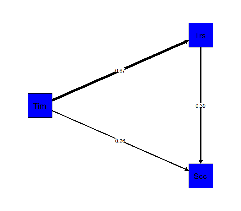

References

Baron, R. M., & Kenny, D. A. (1986). The moderator-mediator variable distinction in social psychological research: Conceptual, strategic, and statistical considerations. Journal of personality and social psychology, 51(6), 1173.

Hallgren, K. A. (2013). Conducting simulation studies in the R programming environment. Tutorials in quantitative methods for psychology, 9(2), 43.

Preacher, K. J., & Hayes, A. F. (2008). Asymptotic and resampling strategies for assessing and comparing indirect effects in multiple mediator models. Behavior research methods, 40(3), 879-891.

Schoemann, A. M., Boulton, A. J., & Short, S. D. (2017). Determining power and sample size for simple and complex mediation models. Social Psychological and Personality Science, 8(4), 379-386.