Partial and Semipartial (part) Correlation

Correlations with 2 or more variables

• Correlations with more than 2 variables present a new challenge
• What if a third variable (X2) actually explains the relationship between X1 and Y?
• We need to find a way to figure out how X2 might relate to X1 and Y!

Example

• Practice Time (X1)
• Performance Anxiety (X2)
• Memory Errors (Y)
• Question, how much does Practice Time and Performance Anxiety predict/explain Memory Errors in performance
• Lets simulate our dataset with the new variables and generate a specific correlation matrix

Variable	Practice Time (X1)	Performance Anxiety (X2)	Memory Errors (Y)
Practice Time (X1)	1	.3	.6
Performance Anxiety (X2)	.3	1	.4
Memory Errors (Y)	.6	.4	1

• Set the mean number for each variable to be 10

#packages we will need to conduct to create and graph our data
library(MASS) #create data
library(car) #graph data
py1 =.6 #Cor between X1 (Practice Time) and Memory Errors
py2 =.4 #Cor between X2 (Performance Anxiety) and Memory Errors
p12= .3 #Cor between X1 (Practice Time) and X2 (Performance Anxiety)
Means.X1X2Y<- c(10,10,10) #set the means of X and Y variables
CovMatrix.X1X2Y <- matrix(c(1,p12,py1,
                            p12,1,py2,
                            py1,py2,1),3,3) # creates the covariate matrix 
#build the correlated variables. Note: empirical=TRUE means make the correlation EXACTLY r. 
# if we say empirical=FALSE, the correlation would be normally distributed around r
set.seed(42)
CorrDataT<-mvrnorm(n=100, mu=Means.X1X2Y,Sigma=CovMatrix.X1X2Y, empirical=TRUE)
#Convert them to a "Data.Frame" & add our labels to the vectors we created
CorrDataT<-as.data.frame(CorrDataT)
colnames(CorrDataT) <- c("Practice","Anxiety","Memory")
#make the scatter plots
scatterplot(Memory~Practice,CorrDataT, smoother=FALSE)
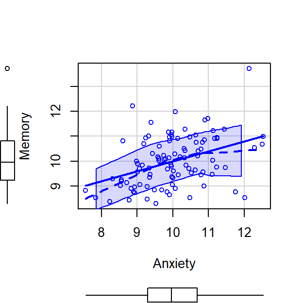
scatterplot(Memory~Anxiety,CorrDataT, smoother=FALSE)
scatterplot(Anxiety~Practice,CorrDataT, smoother=FALSE)
# Pearson Correlations
ry1<-cor(CorrDataT$Memory,CorrDataT$Practice)
ry2<-cor(CorrDataT$Memory,CorrDataT$Anxiety)
r12<-cor(CorrDataT$Anxiety,CorrDataT$Practice)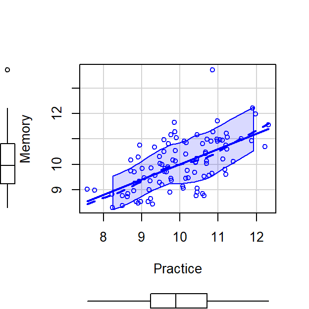

What the problem?

• Practice Time can explain Memory Errors, \(r^2 =\) 0.36
• Anxiety can explain Memory Errors, \(r^2 =\) 0.16
• But how we do know whether Practice Time and Anxiety are explaining the same variance? Anxiety and Practice Time explain each other a little, \(r^2 =\) 0.09

Multiple R

• We use the capital letter, \(R\), now cause we have multiple variables
• \(R_{Y.12} = \sqrt{\frac{r_{Y1}^2 + r_{Y2}^2 - 2r_{Y1} r_{Y2} r_{12}} {1 - r_{12}^2}}\)
• \(R_{Y.12} =\) 0.6427961
• if we square that value, 0.3340659, we get the Multiple \(R^2\)
  • i.e., the total variance explained by these variables on Memory

Semipartial (part) correlation

• We need to define to contribution of each X variable on Y
• Semipartial (also called part) is one of two methods; the other is called partial
  • is called semi, cause it removes the effect of one IV relative to the other without removing the relationship to Y
• Semipartial correlations indicate the “unique” contribution of an independent variable on the dependent variable.
  • When we get to back to regression, “What is the contribution of this X above and beyond the other X variable?”

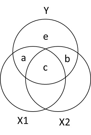
Ballantine for X1, X2, and Y

• \(R_{Y.12}^2 = a + b + c\)
• \(sr_1^2: a = R_{Y.12}^2 - r_{Y2}^2\)
• \(sr_2^2:b = R_{Y.12}^2 - r_{Y1}^2\)

Calcuation

• Calculate unique variance

R2y.12<-sqrt((ry1^2+ry2^2 - (2*ry1*ry2*r12))/(1-r12^2))^2
a = R2y.12 -ry2^2 
b = R2y.12 -ry1^2 

• In other words,
  • In total we explained, 0.4131868 of the Memory Errors
  • Practice Time uniquely explained, 0.2531868 of Memory Errors
  • Anxiety uniquely explained, 0.0531868 of Memory Errors
  • We should not solve for c cause it can be negative (in some weird cases)

Seeing control in action in regression

• Another way to understand it:
  • What if you want to know about Memory Errors and how Practice Time uniquely explains it?
    • Controlling the effect of Anxiety on Practice Time

Memory (Y) ~ Practice(X1) [Control Anxiety (X2)]

1. We can remove the effect of Anxiety on Practice Time by extracting the residuals from lm(X1~X2)
2. Remember the residuals are the leftover (after extracting what was explainable)

scatterplot(Practice~Anxiety,CorrDataT, smoother=FALSE)
CorrDataT$Practice.control.Anxiety<-residuals(lm(Practice~Anxiety, CorrDataT))
scatterplot(Practice.control.Anxiety~Anxiety,CorrDataT, smoother=FALSE)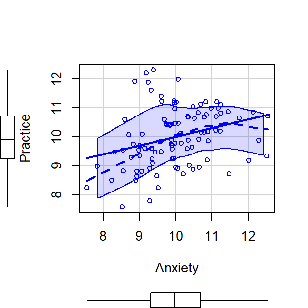

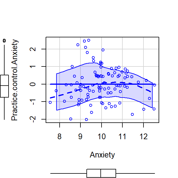
3. Next we can correlate Memory Errors with the residualized Practice Time, cor(Memory,Practice[control Anxiety])

Sr1.alt<-cor(CorrDataT$Memory,CorrDataT$Practice.control.Anxiety)

If we square the correlation value we got 0.5031767, it becomes 0.2531868 which matches our \(a\) from the analysis above.

Memory (Y) ~ Anxiety(X2) [Control Practice (X1)]

1. We can remove effect of Practice on Anxiety by extracting the residuals from lm(X2~X1)
2. Remember the residuals are the leftover (after extracting what was explainable)

scatterplot(Anxiety~Practice,CorrDataT, smoother=FALSE)
CorrDataT$Anxiety.control.Practice<-residuals(lm(Anxiety~Practice, CorrDataT))
scatterplot(Anxiety.control.Practice~Practice,CorrDataT, smoother=FALSE)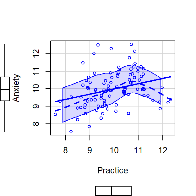

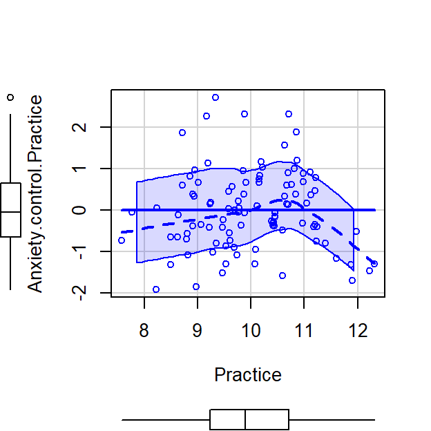
3. Next we can correlate Memory Errors with the residualized Anxiety, cor(Memory,Anxiety[control Practice])

Sr2.alt<-cor(CorrDataT$Memory,CorrDataT$Anxiety.control.Practice)

If we square the correlation value we got 0.2306227, it becomes 0.0531868 which matches our \(b\) from the analysis above.

• In regression when we have more than one predictors they are controlling for each other!

Semipartial notes:

• It can be written as \(sr\) or more specifically, \(sr_1\) for X1 (with X2 removed) and \(sr_2\) (with X1 removed)
• correlations with no control variables are called the zero-order correlations
• in R you can calculate the \(sr\) rather quickly using the ppcor library
• The last variable in the list is the control

library(ppcor)
Sr1<-spcor.test(CorrDataT$Memory, CorrDataT$Practice, CorrDataT$Anxiety)
Sr2<-spcor.test(CorrDataT$Memory, CorrDataT$Anxiety, CorrDataT$Practice)
# Extract result call for Sr1$estimate

• The Semi-partial correlation between Memory and Practice (but controlling for Anxiety) was \(sr\) =0.503
  • If we square it becomes \(sr^2\) = 0.253 which matches our \(a\) from the analysis above.
• The Semi-partial correlation between Memory and Anxiety (but controlling for Practice) was \(sr\) = 0.231
  • If we square it becomes \(sr^2\) = 0.053 which matches our \(b\) from the analysis above.

Relationship to Regression

• Lets say we want to report how practice is related to memory in performance, but we want to control for anxiety?
• The \(sr^2\) for a variable tells us how much \(R^2\) will decrease if that variable is removed from the regression equation
  • Lets test it
  • Lets run 3 regression models (I zscored everything to make the scales all the same)
    • lm(Memory ~ Practice)
    • lm(Memory ~ Anxiety)
      
    • lm(Memory ~ Practice + Anxiety)

# Center variables (if you said scale = TRUE it would zscore the predictors)
CorrDataT$Memory.Z<-scale(CorrDataT$Memory, scale=TRUE, center=TRUE)[,]
CorrDataT$Practice.Z<-scale(CorrDataT$Practice, scale=TRUE, center=TRUE)[,]
CorrDataT$Anxiety.Z<-scale(CorrDataT$Anxiety, scale=TRUE, center=TRUE)[,]
###############Model 1
M.Model.1<-lm(Memory.Z~ Practice.Z, data = CorrDataT)
M.Model.2<-lm(Memory.Z~ Anxiety.Z, data = CorrDataT)
M.Model.3<-lm(Memory.Z~ Practice.Z+Anxiety.Z, data = CorrDataT)

library(stargazer)
stargazer(M.Model.1,M.Model.2,M.Model.3,type="latex",
          intercept.bottom = FALSE, single.row=TRUE, 
          star.cutoffs=c(.05,.01,.001), notes.append = FALSE,
          header=FALSE)

Thus, \[R_{model.3_{P+A}}^2 - sr_{Anxiety}^2 = R^2_{Practice.only}\]

• In R code:

R2.Practice.only = (summary(M.Model.3)$r.squared) - (Sr2$estimate^2)

• So 0.36 = \(R_{Model.1_{Practice}}^2\), as expected

Thus, \[R_{model.3.P+A}^2 - sr_{Practice}^2 = R^2_{Anxiety.only}\]

• In R code:

R2.Anxiety.only = (summary(M.Model.3)$r.squared) - (Sr1$estimate^2)

• So 0.16 = \(R_{Model.2_{Anxiety}}^2\), as expected

Residualized into Regression

• Lets take our residualised effects: Practice (controlling for Anxiety) & Anxiety (controlling for Practice) and compare them to regression model where we enter the two variables into are regression
  • If our regression is semi-partialing we should get the same estimates (if we z-score everything cause residuals we are using are z-scored)

M.Model.4<-lm(Memory.Z~ Practice.control.Anxiety, data = CorrDataT)
M.Model.5<-lm(Memory.Z~ Anxiety.control.Practice, data = CorrDataT)

stargazer(M.Model.3,M.Model.4,M.Model.5,type="latex",
          intercept.bottom = FALSE, single.row=TRUE, 
          star.cutoffs=c(.05,.01,.001), notes.append = FALSE,
          header=FALSE)

• The regression matches our results of when we by-hand residualized

Partial correlation

• Partial correlation asks how much of the Y variance, which is not estimated by the other IVs, is estimated by this variable.

• It removes the shared variance of the control variable (Say X2) from both Y and X1.

• \(pr_1^2: = \frac{a}{a+e} = \frac{R_{Y.12}^2 - r_{Y2}^2}{1-r_{Y2}^2}\)

• \(pr_2^2: \frac{b}{b+e} = \frac{R_{Y.12}^2 - r_{Y1}^2}{1-r_{Y1}^2}\)

Seeing control in action

Another way to understand it:

• What if you want to know about Memory Errors and Practice Time while controlling for Anxiety on both Practice Time and Anxiety (cause Anxiety affect both Memory and Practice Time)
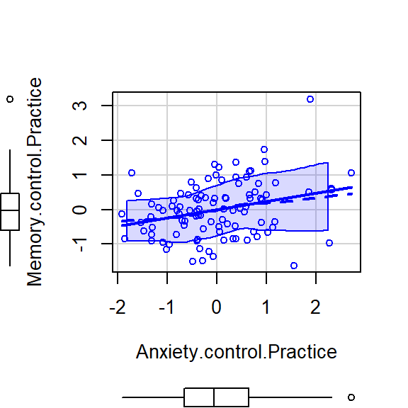
  • We take residuals of lm(Y~X2) and correlate it with the residuals of lm(X1~X2)
    • Remember the residuals are the leftover (after extracting what was explainable)
  • if you want to control for Practice Time you would: residuals of lm(Y~X1) with the residuals of lm(X2~X1)

# Control for Anxiety
CorrDataT$Memory.control.Anxiety<-residuals(lm(Memory~Anxiety, CorrDataT))
CorrDataT$Practice.control.Anxiety<-residuals(lm(Practice~Anxiety, CorrDataT))
scatterplot(Memory.control.Anxiety~Practice.control.Anxiety,CorrDataT, smoother=FALSE)

# Control for Practice Time
CorrDataT$Memory.control.Practice<-residuals(lm(Memory~Practice, CorrDataT))
CorrDataT$Anxiety.control.Practice<-residuals(lm(Anxiety~Practice, CorrDataT))
scatterplot(Memory.control.Practice~Anxiety.control.Practice,CorrDataT, smoother=FALSE)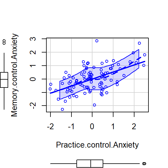

Correlations based on residuals

library(apa)
Res.pr1<-cor_apa(cor.test(CorrDataT$Practice.control.Anxiety,CorrDataT$Memory.control.Anxiety,
                 method = c("pearson")),format ="latex",print = FALSE)
Res.pr2<-cor_apa(cor.test(CorrDataT$Anxiety.control.Practice,CorrDataT$Memory.control.Practice,
                 method = c("pearson")),format ="latex",print = FALSE)

• The pearson correlation Memory (controling for Anxiety) and Practice (controling for Anxiety) was (98)₌.55, _<.001
• The pearson correlation Memory (controling for Practice) and Anxiety (controling for Practice)was (98)₌.29, ₌.004

Correlations based on R Functions

• in R you can calculate the \(pr\) directly via the functions

pr1<-pcor.test(CorrDataT$Memory, CorrDataT$Practice, CorrDataT$Anxiety)
pr2<-pcor.test(CorrDataT$Memory, CorrDataT$Anxiety, CorrDataT$Practice)

• The Partial correlation between Memory (controlling for Anxiety) and Practice (controlling for Anxiety) was \(pr\) =0.55
  • If we square it becomes \(pr^2\) = 0.3
• The Partial correlation between Memory (controlling for Practice) and Anxiety (controlling for Practice) was \(pr\) = 0.29
  • If we square it becomes \(pr^2\) = 0.08
• These values all match our hand residualized calculations

Partial Correlation in Regression?

• What if control for Anxiety?
  • We lose the effect of Anxiety

Partial.Model.1<-lm(Memory.control.Anxiety~ Practice.control.Anxiety+Anxiety.Z, 
                    data = CorrDataT)

stargazer(Partial.Model.1,type="latex",
          intercept.bottom = FALSE, single.row=TRUE, 
          star.cutoffs=c(.05,.01,.001), notes.append = FALSE,
          header=FALSE)

• What if control for Practice?
  • We lose the effect of Practice

  Partial.Model.2<-lm(Memory.control.Practice~ Anxiety.control.Practice+Practice.Z, 
                  data = CorrDataT)
  
  stargazer(Partial.Model.2,type="latex",
        intercept.bottom = FALSE, single.row=TRUE, 
        star.cutoffs=c(.05,.01,.001), notes.append = FALSE,
        header=FALSE)