Regression Review
Linear Regression
- Correlation and regression are similar
- Correlation determines the standardized relationship between X and Y
- Linear regression = 1 DV and 1 IV, where the relationship is a straight line
- Linear regression determines how X predicts Y
- Multiple (linear) regression = 1 DV and 2 + IV (also straight lines)
- Multiple regression determines how X, Z, and etc, predict Y
Modern Regression Equation
- \(Y=B_{YX}X + B_0 + e\)
- \(Y\) = predict value
- \(B_{YX}\) = slope [also can be written as \(B_{1}\) when we get to MR]
- \(B_{0}\) = intercept
- \(e\) = error term (observed - predicted). Also called the residual.
Ice cream example
- We are going to predict happiness scores from the number of spoons
of ice cream.
- Specify the model with the lm function.
set.seed(666)
library(car) #graph data
# 100 people
n <- 100
# Uniform distrobution of Ice Cream scoops
X <- runif(n, 0, 10)
# Slope
Byx<-.6
#intercept
B0 <- 4
# noise
e <- rnorm(n, sd=1.5)
# Our equation to  create Y
Y = Byx*X + B0 + e
#Convert them to a "Data.Frame", which is like SPSS data window
#Built our data frame
IceCreamStudy<-data.frame(Happiness=Y,IceCream=X)
#Extract vectors
IceCream<-IceCreamStudy$IceCream
Happiness<-IceCreamStudy$Happiness
scatterplot(Happiness~IceCream, smoother=FALSE)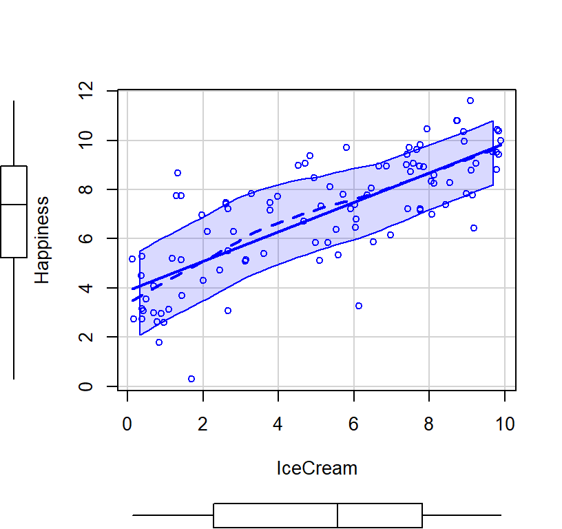
Happy.Model.1<-lm(Happiness~IceCream,data = IceCreamStudy)library(stargazer) # Make APA like tables
stargazer(Happy.Model.1,type="html",
intercept.bottom = FALSE,
single.row=TRUE,
star.cutoffs=c(.05,.01,.001),
notes.append = FALSE,
header=FALSE)| Dependent variable: | |
| Happiness | |
| Constant | 3.895*** (0.301) |
| IceCream | 0.600*** (0.050) |
| Observations | 100 |
| R2 | 0.595 |
| Adjusted R2 | 0.591 |
| Residual Std. Error | 1.551 (df = 98) |
| F Statistic | 144.046*** (df = 1; 98) |
| Note: | p<0.05; p<0.01; p<0.001 |
Intercept
- 3.895 is where the line hit the y-intercept (when happiness = 0).
Slope
- 0.6 is the rise over run
- for each 0.6 change in ice cream value, there is a corresponding change in happiness!
- so we can predict happiness from ice cream score:
(0.6 * 5 spoons of ice cream + baseline happiness intercept: 3.895) = 6.895
- This is your predicted happiness score if you had 5 spoons of ice cream
Error for this prediction?
R will actually do all the prediction for us for each value of ice cream residuals = observed - predicted
- Red dots = observed above predictor line
- Blue dots = observed below predictor line
- the stronger the color, the more an impact that point has in pulling the line in its direction
- Hollow dots = predicted
- The gray lines are the distance between observed and predicted values!
What should the mean of the residuals equal?
# Save the predicted values with our real data
IceCreamStudy$predicted <- predict(Happy.Model.1)
# Save the residual values
IceCreamStudy$residuals <- residuals(Happy.Model.1)

library(ggplot2)  #Fancy pants plotting system
ggplot(data = IceCreamStudy, aes(x = IceCream, y = Happiness)) +
  geom_smooth(method = "lm", se = FALSE, color = "lightgrey") +  # Plot regression slope
  geom_point(aes(color = residuals)) +  # Color mapped here
  scale_color_gradient2(low = "blue", mid = "white", high = "red") +  # Colors to use here
  guides(color = FALSE) +
  geom_segment(aes(xend = IceCream, yend = predicted), alpha = .2) +  # alpha to fade lines
  geom_point(aes(y = predicted), shape = 1) +
  theme_bw()  # Add theme for cleaner look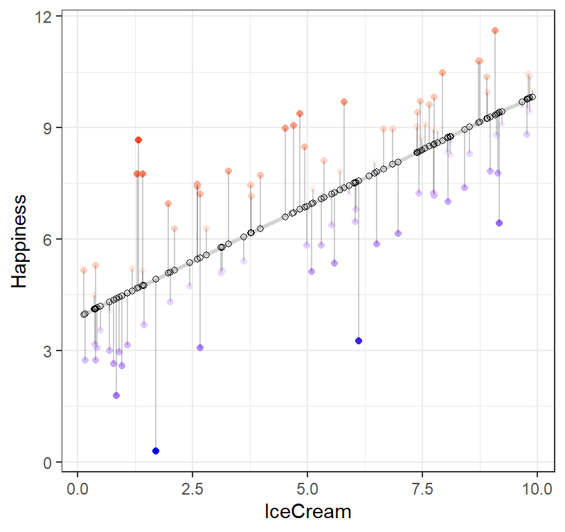
Ordinary least squares (OLS)
- Linear regression finds the best fit line by trying to minimize the sum of the squares of the differences between the observed responses those predicted by the line.
- OLS computationally simple to get the slope value, but is actually inaccurate.
- OLS cannot “fail” to find an answer
\[B_{YX}=\frac{\sum{XY}-\frac{1}{n}\sum{X}\sum{Y}}{\sum{x^2}-\frac{1}{n}\sum{x}^2} = \frac{Cov_{XY}}{var_x}\]
- Mixed-effects models use (ML, REML) to fit. These are more accurate, but can fail (we will return to ML/REML soon).
SE on the terms in the models
- How good is the fit?
- Residual Standard error = \(\sqrt\frac{\sum{e^2}}{n-2}\)
- in R langauge:
n=length(IceCreamStudy$residuals)
RSE = sqrt(sum(IceCreamStudy$residuals^2) / (n-2))- So our error on the prediction is 1.5505018 happiness points based on our model.
SE on the Intercept
- Intercept Standard error = \(RSE\sqrt {\frac{1}{n}+\frac{M_x^2}{(n-1)var_x}}\)
- in R langauge:
ISE = RSE*(sqrt( (1 / n) + (mean(IceCreamStudy$IceCream))^2
/ ((n - 1)*var(IceCreamStudy$IceCream))))- our SE on the intecept is 0.3012578
SE on the Slope
- Intercept Standard error = \(\frac{sd_y}{sd_x}\sqrt{\frac{1 - r_YX^2}{n-2}}\)
- in R language:
#lets extract the r2 from the model
r2.model<-summary(Happy.Model.1)$r.squared
SSE = sd(IceCreamStudy$Happiness)/sd(IceCreamStudy$IceCream) *
sqrt((1- r2.model)/ (n - 2))- SE on the slope is 0.0499665
t-tests on slope and intercept and \(r^2\) value
- Values are tested against 0, so its all one sample t-tests
- slope: \(t = \frac{B_{YX} - H_0}{SE_{B_{YX}}}\)
- intercept: \(t = \frac{B_{0} - H_0}{SE_{B_{0}}}\)
\(r^2\) is a little different as its a correlation value
- correlations are not normally distributed
- Fisher created a coversion for r to make it a z (called Fishers’ \(r\) to \(Z\))
- \(r^2\): \(t = \frac{r_{XY}\sqrt{n-2}-H_0}{\sqrt{1-r_{XY}^2}}\) , where \(df = n - 2\)
- its often given for as an F value, remember \(t = F^2\)
#intercept
t.I= Happy.Model.1$coefficients[1]/ISE
#Slope
t.S= Happy.Model.1$coefficients[2]/SSE
# For r-squared
t.r2xy = r2.model^.5*sqrt(n-2)/sqrt(1-r2.model)
F.r2xy = t.r2xy^2- Intercept t = 12.929604
- Slope t = 12.0018969
- \(R^2\) F-test = 144.0455294
- Note: We are testing null hypothesis value for slope, i.e., null = 0. But it’s a terrible guess. Everything correlates with everything, so it’s important to keep this in mind moving forward.
Regression in ANOVA format
- You can also report the results of all the predictors (if you have multiple) in ANOVA style format (F-test we calculated above on \(R^2\))
- This is useful in multiple regression as it tell your if your overall set of predictors is significant
anova(Happy.Model.1)## Analysis of Variance Table
##
## Response: Happiness
## Df Sum Sq Mean Sq F value Pr(>F)
## IceCream 1 346.29 346.29 144.05 < 2.2e-16 ***
## Residuals 98 235.60 2.40
## ---
## Signif. codes: 0 '***' 0.001 '**' 0.01 '*' 0.05 '.' 0.1 ' ' 1Multiple Regresion
With No Redundancy
- Predictors do not correlate with each other
- Ice cream spoons (X1)
- Brownies squares (X2)
- Happiness score (Y)
- We will assume ice cream and brownies are unqiue predictors of happiness
- Note: The simulations are based on multivariate functions now so we can control the relationships between the variables very carefully.
- We will set a mean for each at 5 and create a covariance matrix between the variables
\[ \mathbf{Cov} = \sigma^2\left[\begin{array} {rrr} 1 & 0 & .6 \\ 0 & 1 & .4 \\ .6 & .4 & 1 \end{array}\right] \] where, \(\sigma^2 = 4\)
- tow column order
- Ice cream, 2. Brownines, 3. Happiness
- Simulation below:
library(MASS) # use multivariate norm function to better control relationships
py1 =.6 #Cor between X1 (ice cream) and happiness
py2 =.4 #Cor between X2 (Brownies) and happiness
p12 = 0 #Cor between X1 (ice cream) and X2 (Brownies)
Means.X1X2Y<- c(5,5,5) #set the means of X and Y variables
CovMatrix.X1X2Y <- matrix(c(1,p12,py1,
                            p12,1,py2,
                            py1,py2,1),3,3)*4 # creates the covariate matrix
#build the correlated variables. Note: empirical=TRUE means make the correlation EXACTLY r.
# if we say empirical=FALSE, the correlation would be normally distributed around r
set.seed(666)
CorrDataT<-mvrnorm(n=100, mu=Means.X1X2Y,Sigma=CovMatrix.X1X2Y, empirical=TRUE)
#Covert them to a "Data.Frame", which is like SPSS data window
CorrDataT<-as.data.frame(CorrDataT)
#lets add our labels to the vectors we created
colnames(CorrDataT) <- c("IceCream","Brownies","Happiness")
CorrDataT$Happiness<-CorrDataT$Happiness
# Correlations
ry1<-cor(CorrDataT$Happiness,CorrDataT$IceCream)
ry2<-cor(CorrDataT$Happiness,CorrDataT$Brownies)
r12<-cor(CorrDataT$Brownies,CorrDataT$IceCream)- Run model and report results
###############Model 1
Ice.Model<-lm(Happiness~ IceCream, data = CorrDataT)
###############Model 2
Ice.Brown.Model<-lm(Happiness~ IceCream+Brownies, data = CorrDataT)
stargazer(Ice.Model,Ice.Brown.Model,type="html",
         column.labels = c("Model 1", "Model 2"),
          intercept.bottom = FALSE,
          single.row=TRUE,
          star.cutoffs=c(.05,.01,.001),
          notes.append = FALSE,
header=FALSE)| Dependent variable: | ||
| Happiness | ||
| Model 1 | Model 2 | |
| (1) | (2) | |
| Constant | 2.000*** (0.435) | -0.000 (0.517) |
| IceCream | 0.600*** (0.081) | 0.600*** (0.070) |
| Brownies | 0.400*** (0.070) | |
| Observations | 100 | 100 |
| R2 | 0.360 | 0.520 |
| Adjusted R2 | 0.353 | 0.510 |
| Residual Std. Error | 1.608 (df = 98) | 1.400 (df = 97) |
| F Statistic | 55.125*** (df = 1; 98) | 52.542*** (df = 2; 97) |
| Note: | p<0.05; p<0.01; p<0.001 | |
#packages we will need to plot our results
library(effects)
#plot individual effects
Ice.Brown.Model.Plot <- allEffects(Ice.Brown.Model,
xlevels=list(IceCream=seq(0, 10, 1),
Brownies=seq(0, 10, 1)))
plot(Ice.Brown.Model.Plot,
'IceCream', ylab="Happiness")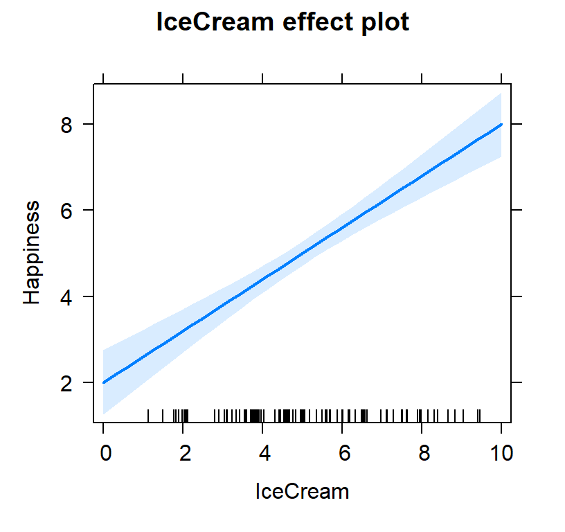
plot(Ice.Brown.Model.Plot,
     'Brownies', ylab="Happiness")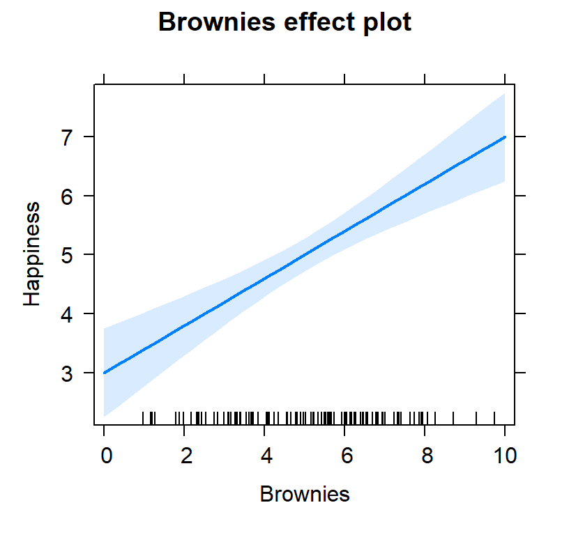
#plot both effects
Ice.Brown.Model.Plot2<-Effect(c("IceCream", "Brownies"),
                              Ice.Brown.Model,
                              xlevels=list(IceCream=c(0, 10),
                                           Brownies=c(0,10)))
plot(Ice.Brown.Model.Plot2)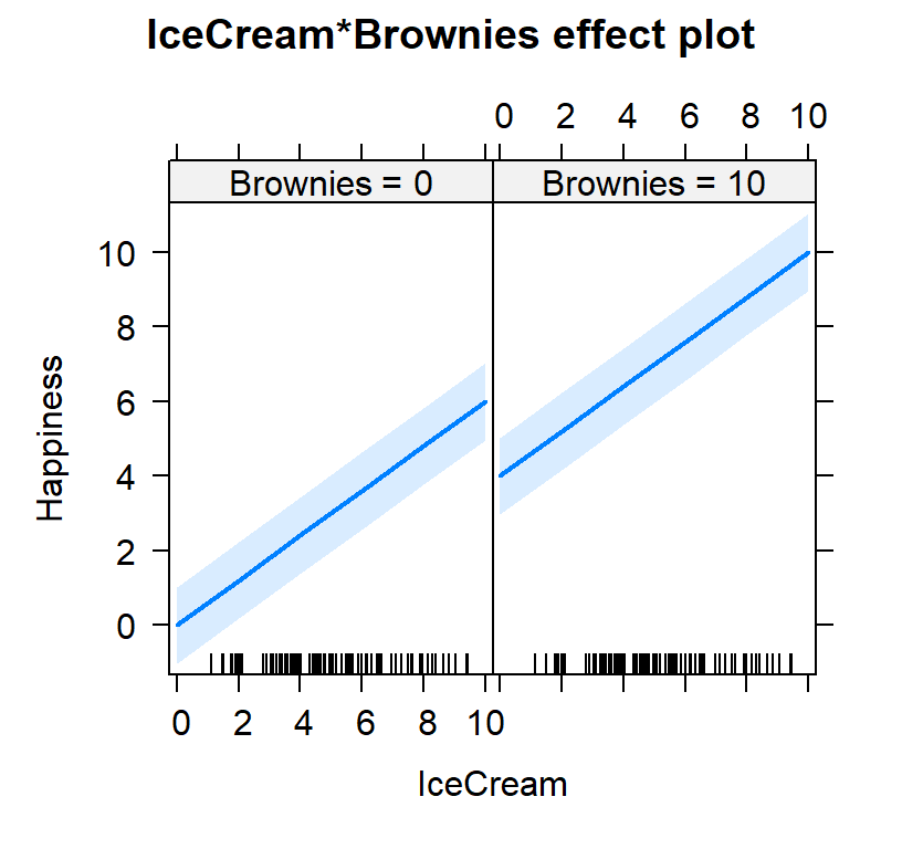
Intercept
- Why did my intercept change?
- Intercept is the 0 point for ice cream and 0 brownies.
- See the figure above for the new intercept when both predictors are in the model
- We can fix the problem by centering our predictors [scale function]
# Center variables (if you said scale = TRUE it would zscore the predictors)
CorrDataT$IceCream.C<-scale(CorrDataT$IceCream, scale=FALSE, center=TRUE)[,]
CorrDataT$Brownies.C<-scale(CorrDataT$Brownies, scale=FALSE, center=TRUE)[,]
###############Model 1 Centered
Ice.Model.C<-lm(Happiness~ IceCream.C, data = CorrDataT)
###############Model C Centered
Ice.Brown.Model.C<-lm(Happiness~ IceCream.C+Brownies.C, data = CorrDataT)
stargazer(Ice.Model.C,Ice.Brown.Model.C,type="html",
column.labels = c("Model 1", "Model 2"),
intercept.bottom = FALSE,
single.row=TRUE,
star.cutoffs=c(.05,.01,.001),
notes.append = FALSE,
header=FALSE)| Dependent variable: | ||
| Happiness | ||
| Model 1 | Model 2 | |
| (1) | (2) | |
| Constant | 5.000*** (0.161) | 5.000*** (0.140) |
| IceCream.C | 0.600*** (0.081) | 0.600*** (0.070) |
| Brownies.C | 0.400*** (0.070) | |
| Observations | 100 | 100 |
| R2 | 0.360 | 0.520 |
| Adjusted R2 | 0.353 | 0.510 |
| Residual Std. Error | 1.608 (df = 98) | 1.400 (df = 97) |
| F Statistic | 55.125*** (df = 1; 98) | 52.542*** (df = 2; 97) |
| Note: | p<0.05; p<0.01; p<0.001 | |
- The table now matches our simulation perfectly
Multiple R
- We use the capital letter, \(R\), now cause we have multiple X variables
- \(R_{Y.12} = \sqrt{\frac{r_{Y1}^2 + r_{Y2}^2 - 2r_{Y1} r_{Y2} r_{12}} {1 - r_{12}^2}}\)
- \(R_{Y.12} =\) 0.7211103
- if we square that value, 0.52, we get the Multiple \(R^2\)
- or the total variance explained by these variables on happiness
Estimating population R-squared
- \(\rho^2\) is estimated by multiple \(R^2\)
- Problem: in small samples correlations are unstable (and inflated)
- Also, as we add predictors, \(R^2\) gets inflated
- So we use an adjusted multiple \(R^2\)
- Adjusted \(R^2 = 1 - 1- R_Y^2 \frac{n-1}{n-k-1}\)
Partial Redundancy
- Regressions/correlations with more than 2 variables often presentes
a new challenge
- What if a third variable (X2) actually explains the relationship between X1 and Y?
- We need to find a way to figure out how X2 might relate to X1 and Y!
- In short: What happens if the predictors did correlate with each other?
- New question: How much does ice cream and brownies predict/explain happiness scores given ice cream and bronwies correlate with each other?
\[ \mathbf{Cov} = \sigma^2\left[\begin{array} {rrr} 1 & .3 & .6 \\ .3 & 1 & .4 \\ .6 & .4 & 1 \end{array}\right] \] where, \(\sigma^2 = 4\)
- Row/column order
- Ice cream, 2. Brownines, 3. Happiness
- Simulation below:
library(MASS) #create data
py1 =.6 #Cor between X1 (ice cream) and happiness
py2 =.4 #Cor between X2 (Brownies) and happiness
p12= .3 #Cor between X1 (ice cream) and X2 (Brownies)
Means.X1X2Y<- c(5,5,5) #set the means of X and Y variables
CovMatrix.X1X2Y <- matrix(c(1,p12,py1,
                            p12,1,py2,
                            py1,py2,1),3,3)*4 # creates the covariate matrix
set.seed(42)
CorrDataT2<-mvrnorm(n=100, mu=Means.X1X2Y,Sigma=CovMatrix.X1X2Y, empirical=TRUE)
#Convert them to a "Data.Frame", which is like SPSS data window
CorrDataT2<-as.data.frame(CorrDataT2)
#lets add our labels to the vectors we created
colnames(CorrDataT2) <- c("IceCream","Brownies","Happiness")
# Pearson Correlations
ry1<-cor(CorrDataT2$Happiness,CorrDataT2$IceCream)
ry2<-cor(CorrDataT2$Happiness,CorrDataT2$Brownies)
r12<-cor(CorrDataT2$Brownies,CorrDataT2$IceCream)
What the problem?
- Ice Cream can explain happiness, \(r^2 =\) 0.36
- Brownies can explain happiness, \(r^2 =\) 0.16
- But how we do know whether Ice Cream and Brownies are explaining the same variance? Brownies and Ice Cream explain each other a little, \(r^2 =\) 0.09
Impacts on regression
- The slope for Ice cream should be B1 = 0.6
- The slope for Brownies should be B2 = 0.4
- but we know from the simulation that Ice cream and Brownies correlate, \(r =\) 0.3
# Center variables (if you said scale = TRUE it would zscore the predictors)
CorrDataT2$IceCream.C<-scale(CorrDataT2$IceCream, scale=FALSE, center=TRUE)[,]
CorrDataT2$Brownies.C<-scale(CorrDataT2$Brownies, scale=FALSE, center=TRUE)[,]
###############Model 1 Centered
Ice.Model.C2<-lm(Happiness~ IceCream.C, data = CorrDataT2)
###############Model C Centered
Ice.Brown.Model.C2<-lm(Happiness~ IceCream.C+Brownies.C, data = CorrDataT2)
stargazer(Ice.Model.C2,Ice.Brown.Model.C2,type="html",
column.labels = c("Model 1", "Model 2"),
intercept.bottom = FALSE, single.row=TRUE,
star.cutoffs=c(.05,.01,.001), notes.append = FALSE,
header=FALSE)| Dependent variable: | ||
| Happiness | ||
| Model 1 | Model 2 | |
| (1) | (2) | |
| Constant | 5.000*** (0.161) | 5.000*** (0.155) |
| IceCream.C | 0.600*** (0.081) | 0.527*** (0.082) |
| Brownies.C | 0.242** (0.082) | |
| Observations | 100 | 100 |
| R2 | 0.360 | 0.413 |
| Adjusted R2 | 0.353 | 0.401 |
| Residual Std. Error | 1.608 (df = 98) | 1.548 (df = 97) |
| F Statistic | 55.125*** (df = 1; 98) | 34.150*** (df = 2; 97) |
| Note: | p<0.05; p<0.01; p<0.001 | |
- The slopes do not match the simulation slopes
Semipartial (part) correlation
- We need to define to contribution of each X variable on Y
- Semipartial (also called part) is one of two methods, the other is called partial
- is called semi, cause it removes the effect of one IV relative to the other without removing the relationship to Y
- Semipartial correlations indicate the “unique” contribution of an independent variable.
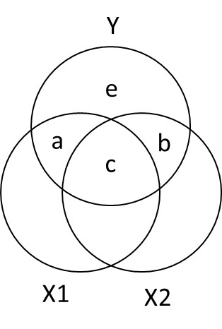
Ballantine for X1, X2, and Y
- \(R_{Y.12}^2 = a + b + c\)
- \(sr_1^2: a = R_{Y.12}^2 - r_{Y2}^2\)
- \(sr_2^2:b = R_{Y.12}^2 - r_{Y1}^2\)
Calcuation
- Calcuate unique varience
R2y.12<-sqrt((ry1^2+ry2^2 - (2*ry1*ry2*r12))/(1-r12^2))^2
  a = R2y.12 -ry2^2
b = R2y.12 -ry1^2 - in other words,
- In total we explained, 0.4131868 of the happiness ratings (matches our \(R^2\) values from the regression table above)
- ice cream uniquely explained, 0.2531868 of happiness ratings
- brownies uniquely explained, 0.0531868 of happiness ratings
- We should not solve for c cause it can be negative (in some cases)
Seeing control in action in regression
- Another way to understand it:
- What if you want to know about happiness and how ice cream uniquely explains it? [controling the effect of brownies on ice cream]
- We can remove affect of brownies on ice cream by extracting the residuals lm(X1~X2)
- Remember the residuals are the left over (after extracting what was explainable)
- Next we can correlate happiness with the residualized ice cream.
#control for brownies
CorrDataT2$Ice.control.Brownies<-residuals(lm(IceCream~Brownies, CorrDataT2))
Sr1.alt<-cor(CorrDataT2$Ice.control.Brownies,CorrDataT2$Happiness)
If we sqaure the correlation value we got 0.5031767, it becomes 0.2531868 which matches our \(a\) from the analysis above.
- We can repeat this analysis but changing our control to find \(b\).
#control for ice cream
CorrDataT2$Brownies.control.Ice<-residuals(lm(Brownies~IceCream, CorrDataT2))
Sr2.alt<-cor(CorrDataT2$Happiness,CorrDataT2$Brownies.control.Ice)
If we sqaure the correlation value we got 0.2306227, it becomes 0.0531868 which matches our \(b\) from the analysis above.
- Thus in regression when we have more than one predictors they are controling for each other!
Relative importance
- There is a package that will do most of tht work for us
- The function calc.relimp in relaimpo has
lots of paramaters
- first would be if we entered them one at time
- last matches are semipartialed results (but order can matter)
library(relaimpo)
 crlm <- calc.relimp(Ice.Brown.Model.C2,
                     type = c("first","last"), rela = FALSE )
 crlm
## Response variable: Happiness
## Total response variance: 4
## Analysis based on 100 observations
##
## 2 Regressors:
## IceCream.C Brownies.C
## Proportion of variance explained by model: 41.32%
## Metrics are not normalized (rela=FALSE).
##
## Relative importance metrics:
##
## last first
## IceCream.C 0.25318681 0.36
## Brownies.C 0.05318681 0.16Full Redundancy (Spurious models)
- when, \(r_{Y2} \approx r_{Y1}r_{12}\)
- X1 is confounded in X2
- X1 and X2 are completely redundant
\[ \mathbf{Cov} = \sigma^2\left[\begin{array} {rrr} 1 & .99 & .6 \\ .99 & 1 & .6 \\ .6 & .6 & 1 \end{array}\right] \] where, \(\sigma^2 = 4\)
- Row/column order
- Oreos, 2. Cookies, 3. Happiness
- Simulation below:
library(MASS) # use multivariate norm function to better control relationships
I.py1 =.6 #Cor between X1 Oreos and happiness
I.py2 =.6 #Cor between X2 Cookies and happiness
I.p12 = .99 #Cor between X1 Oreos and X2 Cookies
I.Means.X1X2Y<- c(0,0,0) #set the means of X and Y variables
I.CovMatrix.X1X2Y <- matrix(c(1,I.p12,I.py1,
                            I.p12,1,I.py2,
                            I.py1,I.py2,1),3,3)*4 # creates the covariate matrix
set.seed(42)
IData<-mvrnorm(n=100, mu=I.Means.X1X2Y,Sigma=I.CovMatrix.X1X2Y, empirical=TRUE)
#Covert them to a "Data.Frame", which is like SPSS data window
IData<-as.data.frame(IData)
#lets add our labels to the vectors we created
colnames(IData) <- c("Oreos","Cookies","Happiness")
###############Model 1
Oreos.model<-lm(Happiness~ Oreos, data = IData)
###############Model 2
Cookies.model<-lm(Happiness~ Cookies, data = IData)
###############Model 3
Oreos.cookies.model<-lm(Happiness~ Oreos+Cookies, data = IData)
stargazer(Oreos.model,Cookies.model,Oreos.cookies.model,type="html",
column.labels = c("Oreos", "Cookies","Oreos+Cookies" ),
intercept.bottom = FALSE,
single.row=TRUE,
star.cutoffs=c(.05,.01,.001),
notes.append = FALSE,
header=FALSE)| Dependent variable: | |||
| Happiness | |||
| Oreos | Cookies | Oreos+Cookies | |
| (1) | (2) | (3) | |
| Constant | -0.000 (0.161) | -0.000 (0.161) | -0.000 (0.161) |
| Oreos | 0.600*** (0.081) | 0.302 (0.575) | |
| Cookies | 0.600*** (0.081) | 0.302 (0.575) | |
| Observations | 100 | 100 | 100 |
| R2 | 0.360 | 0.360 | 0.362 |
| Adjusted R2 | 0.353 | 0.353 | 0.349 |
| Residual Std. Error | 1.608 (df = 98) | 1.608 (df = 98) | 1.614 (df = 97) |
| F Statistic | 55.125*** (df = 1; 98) | 55.125*** (df = 1; 98) | 27.496*** (df = 2; 97) |
| Note: | p<0.05; p<0.01; p<0.001 | ||
Suppression
- Suppression is a strange case where the IV -> DV relationship is hidden (suppressed) by another variable
- Tax cuts cause growth, tax cuts cause inflation. Tax cuts alone might look +, but add in inflation and now tax cuts could make cause the growth to look different
- Or the the suppressor variable can cause a flip in the sign of the relationship
- Here is an example where the effect was hidden:
sup.py1 =  2.5 #Covar between tax cuts and growth
sup.py2 = -5.5 #Covar between inflation and growth
sup.p12 =  4  #Covar between tax cuts and inflation

Supp.X1X2Y<- c(5,5,5) #set the means of X and Y variables
Supp.CovMatrix.X1X2Y <- matrix(c(10,sup.p12,sup.py1,
                                 sup.p12,10,sup.py2,
                                 sup.py1,sup.py2,10),3,3) # creates the covariate matrix

set.seed(42)
SuppData<-mvrnorm(n=100, mu=Supp.X1X2Y,Sigma=Supp.CovMatrix.X1X2Y, empirical=TRUE)

#Covert them to a "Data.Frame"
SuppData<-as.data.frame(SuppData)
colnames(SuppData) <- c("TaxCuts","inflation","growth")

###############Model 1
TaxCutsOnly<-(lm(growth~ TaxCuts, data = SuppData))
###############Model 2
Full.Model<-lm(growth~ TaxCuts+inflation, data = SuppData)
stargazer(TaxCutsOnly,Full.Model,type="html",
column.labels = c("TaxCutsOnly", "Full.Model"),
intercept.bottom = FALSE,
single.row=TRUE,
star.cutoffs=c(.05,.01,.001),
notes.append = FALSE,
header=FALSE)| Dependent variable: | ||
| growth | ||
| TaxCutsOnly | Full.Model | |
| (1) | (2) | |
| Constant | 3.750*** (0.578) | 6.071*** (0.452) |
| TaxCuts | 0.250* (0.098) | 0.560*** (0.073) |
| inflation | -0.774*** (0.073) | |
| Observations | 100 | 100 |
| R2 | 0.063 | 0.565 |
| Adjusted R2 | 0.053 | 0.557 |
| Residual Std. Error | 3.077 (df = 98) | 2.106 (df = 97) |
| F Statistic | 6.533* (df = 1; 98) | 63.116*** (df = 2; 97) |
| Note: | p<0.05; p<0.01; p<0.001 | |
- You will notice tax cuts alone, 0.25, was lower than 0.5595238 controlling for inflation.
- However, you will notice inflation,-0.7738095, has a bigger effect (and negative) effect than tax cuts 0.5595238
- So in other words, yes tax cuts work but they don’t override inflation!
Lets try to graph our predictions
- Challenge is that we need to account for 2 predictors now.
- So simple scatter plots will not work
- Also how you plot depends on your theory/experiment/story
- We need to control for inflation (or view tax slope at different levels of inflation)
- First lets view the tax slope without controlling for inflation
#plot individual effects
Tax.Model.Plot <- allEffects(TaxCutsOnly, xlevels=list(TaxCuts=seq(3, 7, 1)))
plot(Tax.Model.Plot, 'TaxCuts', ylab="Growth")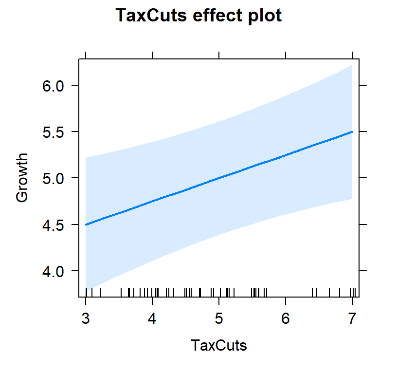
- Now lets view it controlling for inflation
#plot individual effects
Full.Model.Plot <- allEffects(Full.Model, xlevels=list(TaxCuts=seq(3, 7, 1),inflation=seq(3, 7, 1)))
plot(Full.Model.Plot, 'TaxCuts', ylab="Growth")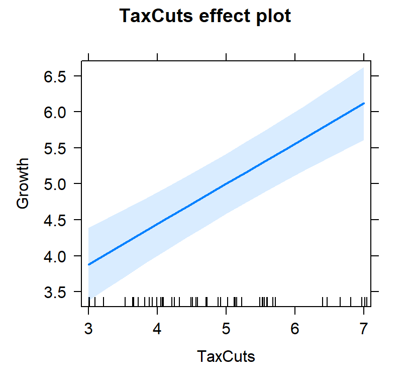
plot(Full.Model.Plot, 'inflation', ylab="Growth")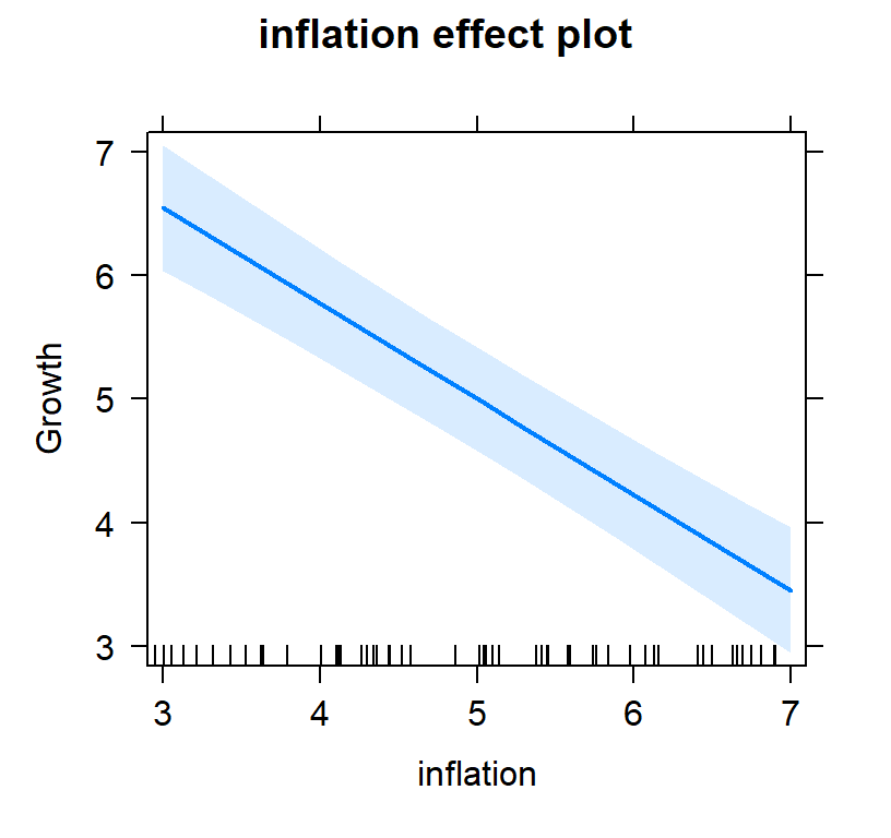
#plot both effects
Full.Model.Plot2<-Effect(c("TaxCuts", "inflation"), Full.Model,xlevels=list(TaxCuts=c(3, 7), inflation=c(3,7)))
plot(Full.Model.Plot2)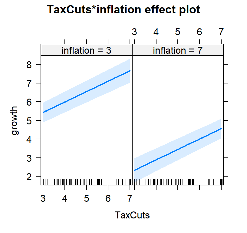
Multiple Linear Regression Assumptions
Multicollinearity: Predictors cannot be fully (or nearly fully) redundant [check the correlations between predictors]
Homoscedasticity of residuals to fitted values
Normal distribution of residuals
Absence of outliers
Ratio of cases to predictors
- Number of cases must exceed the number of predictors
- Barely acceptable minimum: 5 cases per predictor
- Preferred minimum: 20-30 cases per predictor
- This is all subject to a power analysis
Linearity of prediction
Independence (no auto-correlated errors)
Fast and dirty method to check some of the assumptions
- Its better to just plot your data, but its fun fast check
Too see them all go to http://ademos.people.uic.edu/Chapter12.html
layout(matrix(c(1,2,3,4),2,2))
plot(Full.Model)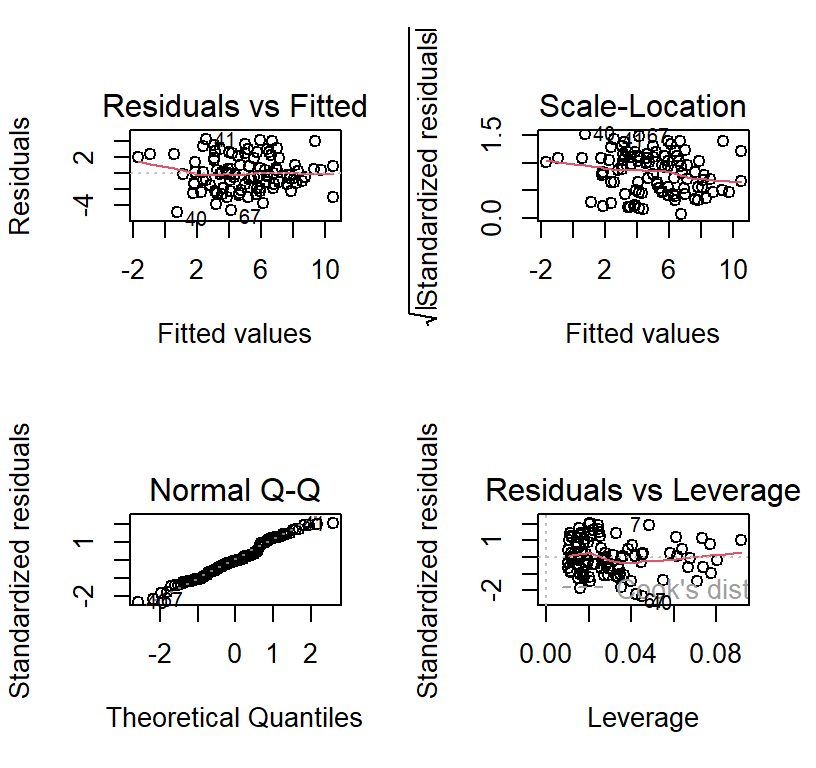
library(gvlma)
Full.Model.Assumptions <- gvlma(Full.Model)
summary(Full.Model.Assumptions)
##
## Call:
## lm(formula = growth ~ TaxCuts + inflation, data = SuppData)
##
## Residuals:
## Min 1Q Median 3Q Max
## -4.805 -1.386 -0.138 1.677 4.202
##
## Coefficients:
## Estimate Std. Error t value Pr(>|t|)
## (Intercept) 6.07143 0.45203 13.431 < 2e-16 ***
## TaxCuts 0.55952 0.07303 7.662 1.39e-11 ***
## inflation -0.77381 0.07303 -10.596 < 2e-16 ***
## ---
## Signif. codes: 0 '***' 0.001 '**' 0.01 '*' 0.05 '.' 0.1 ' ' 1
##
## Residual standard error: 2.106 on 97 degrees of freedom
## Multiple R-squared: 0.5655, Adjusted R-squared: 0.5565
## F-statistic: 63.12 on 2 and 97 DF, p-value: < 2.2e-16
##
##
## ASSESSMENT OF THE LINEAR MODEL ASSUMPTIONS
## USING THE GLOBAL TEST ON 4 DEGREES-OF-FREEDOM:
## Level of Significance = 0.05
##
## Call:
## gvlma(x = Full.Model)
##
## Value p-value Decision
## Global Stat 2.3081 0.6793 Assumptions acceptable.
## Skewness 0.1939 0.6597 Assumptions acceptable.
## Kurtosis 1.4644 0.2262 Assumptions acceptable.
## Link Function 0.4897 0.4841 Assumptions acceptable.
## Heteroscedasticity 0.1600 0.6891 Assumptions acceptable.Interactions
- Interactions have the same meaning they did in ANOVA
- there is a synergistic effect between two variables
- However now we can examine interactions between continuous variables
- Additive Effects
\[Y = B_1X + B_2Z + B_0\]
- Interactive Effects:
\[Y = B_1X + B_2Z + B_3XZ + B_0\]
Example of Interaction
- We need to make multivariate set of variables and then force an interaction
- DV: Reading comprehension, IVs: Age + IQ
- These are not all mean centered because of interpretation
library(car)
set.seed(12345)
# 250 people
n <- 250
# Uniform distrobution of Ages (5 to 15 year olds), but 5 = 0 point
X <- runif(n, 0, 10)
# Centered normal distrobution of IQ (100 +-15)
Z <- rnorm(n, 0, 15)
e <- rnorm(n, 0, sd=10)
# Our equation to  create Y
Y = .1*X + .25*Z + .1*X*Z + 50 + e
#Built our data frame
Reading.Data<-data.frame(ReadingComp=Y,Age=X,IQ=Z)
Lets test an interaction
- Model 1: Examine a main-effects model (X + Z) [not necessary but useful]
- Model 2: Examine a main-effects + Interaction model (X + Z + X:Z)
- Note: You can simply code it as X*Z in r, as it will automatically do (X + Z + X:Z)
#models
Centered.Read.1<-lm(ReadingComp~Age+IQ,Reading.Data)
Centered.Read.2<-lm(ReadingComp~Age*IQ,Reading.Data)

stargazer(Centered.Read.1,Centered.Read.2,type="html",
          column.labels = c("Main Effects", "Interaction"),
          intercept.bottom = FALSE, single.row=TRUE,
          star.cutoffs=c(.05,.01,.001), notes.append = FALSE,
header=FALSE)| Dependent variable: | ||
| ReadingComp | ||
| Main Effects | Interaction | |
| (1) | (2) | |
| Constant | 47.710*** (1.388) | 48.288*** (1.312) |
| Age | 0.546* (0.225) | 0.440* (0.213) |
| IQ | 0.817*** (0.045) | 0.333*** (0.095) |
| Age:IQ | 0.085*** (0.015) | |
| Observations | 250 | 250 |
| R2 | 0.582 | 0.630 |
| Adjusted R2 | 0.578 | 0.626 |
| Residual Std. Error | 10.266 (df = 247) | 9.670 (df = 246) |
| F Statistic | 171.653*** (df = 2; 247) | 139.732*** (df = 3; 246) |
| Note: | p<0.05; p<0.01; p<0.001 | |
- Also change in \(R^2\) is significant, as we might expect
ChangeInR<-anova(Centered.Read.1,Centered.Read.2)
ChangeInR
## Analysis of Variance Table
##
## Model 1: ReadingComp ~ Age + IQ
## Model 2: ReadingComp ~ Age * IQ
## Res.Df RSS Df Sum of Sq F Pr(>F)
## 1 247 26029
## 2 246 23005 1 3024 32.336 3.665e-08 ***
## ---
## Signif. codes: 0 '***' 0.001 '**' 0.01 '*' 0.05 '.' 0.1 ' ' 1How visualize this?
- Well, there are some options
- We can do a fancy-pants surface plot, but that is hard to put into a paper
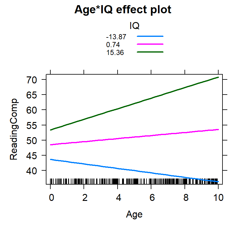
- More common this is to examine slope of one factor at different levels of the other (Simple Slopes)
- What we need to decide is at which levels
Based on the SD
- We select 3 values: \(M-1SD\), \(M\), \(M+1SD\)
- Not it does not have to be 1 SD, it can be 1.5,2 or 3
- Assumes normality for IV
IQ.SD<-c(mean(Reading.Data$IQ)-sd(Reading.Data$IQ),
         mean(Reading.Data$IQ),
         mean(Reading.Data$IQ)+sd(Reading.Data$IQ))
IQ.SD<-round(IQ.SD,2)
IQ.SD
## [1] -13.87 0.74 15.36Inter.1c<-effect(c("Age*IQ"), Centered.Read.2,
xlevels=list(Age=seq(0,10, 1),
IQ=IQ.SD))
plot(Inter.1c, multiline = TRUE)