Moments, Z-scores, Probability, & Sampling Error

Gaussian Distribution

Gaussian distribution (named after Johann Carl Friedrich Gauss, 1777-1855, aka the normal distribution) is a special distribution that is the basis of Classical Parametric Statistics, why? Well because its really easy to work with (not a joke). It is defined by and it is defined by 2 parameters (\(\mu\) & \(\sigma\)) when the other two parameters (Skewness & Kurtosis) equal 0. I will come back to those below under Moments.

Gaussian distribution (aka the normal distribution) will serve as our population distribution. R will let us simulate a population with \(\mu = 100; \sigma = 15; N = 1e10^6\). Note: the seed allows all have to identical random results.

We will use the rnorm function which will allow us to pass the parameters we want to use to create our population distribution. As R is an object-oriented language, the results of this function will be an object (a bucket, which we filled with random, but normally distributed numbers). We can examine what is in this object, but first we must name out this object, and we call it anything we want as long as we don’t have spaces in our name (for example, The.Bucket.of.Many.Random.Numbers, however that is a silly name), so we will call it Normal.Sample.1.

set.seed(666)
n=1e6 #1 million people
Mu=100 # Set pop mean
S = 15 # set pop SD
Normal.Sample.1<-rnorm(n, mean = Mu, sd = S)

We can add a histogram (hist), where we could define a bin size (but R will do it automatically if we do not pass one) and add labels, as all graphs should be well labeled.

hist(Normal.Sample.1,
  main="Raw Score Histogram", 
  xlab="Population Distribution", ylab="Frequency")
abline(v=100, col="black")

As we can see in Figure above, we have what seems a nice normal distribution with 1 million random scores. Next, we need to examine the shape of the distribution by looking at the 4 moments.

Moments

There are 4 moments that can capture important aspects of the distribution (1. center, 2. spread, 3.symmetry, and 4. peakiness).

Moment 1: Central Tendency

Captures the center of the distribution and be defined three classical ways (Mean, Median, Mode). Mean/Median/Mode are used to identify a single score (point-estimation) that is representative for an entire distribution or set of data.

Mean (the average):

• is the standard measure of central tendency in statistics.
• is not necessarily equal to any score in the data set
• is the most stable measure from sample to sample.
• is very influenced by outliers (the mean will be strongly influenced by the presence of extreme scores).
• is based on all scores from the sample but the mode and the median are not.

Median (the middle number):

• is not sensitive to outliers!
• is the best measure of central tendency if the distribution is skewed.

Mode (most common number):

• is the least stable measure from sample to sample.

Mean

In R there many ways to do things. There are often packages which people have created to make your life easier but let’s start by replicating the formula in code. You will notice below that code that we can write it multiple steps, or we could have done it all at once. But first sum the object and divide it by the length of the object (note that length is the way we tabulate how long our object is. In this case out object is a vector: which is a simply a 1-dim string of numbers).

\[M = \frac{\Sigma X}{N}\]

Note: In R you can use “=” or “<-” to create the object. To help make the code more readable I use “=” to set argument or parameters that I pass into function and “<-” for objects. R coders in general use “<-”.

SumX <- sum(Normal.Sample.1) # Sum of X
N <- length(Normal.Sample.1) # length of vector 
M <- SumX/N # calc mean
M # Calls objects for us to see

## [1] 99.99483

# OR all at once
M <-sum(Normal.Sample.1)/length(Normal.Sample.1)

The mean was 99.99 and close to expected \(\mu\) of 100. However, we should use the built-in function, mean(Normal.Sample.1)

Median

Here I can call median and not create an object. This will cause R to show me the answer, but not save it.

median(Normal.Sample.1)

## [1] 99.98384

Mode

There is no built-in mode function in R that gives the mode. Note: The function mode yields information about the type of data (numeric, factor, etc.) of the object. So you have to go to google and either 1) find a package or 2) find someone who wrote a function.

• Why is the mode a problem? Because it might be multi-modal or non-modal.

• Online people suggest the modeest package. However, this package has not been updated to work in the latest version R (3.6.1 as of 8-2019).

• When packages fail, we turn to stackoverflow. You can follow this link and see all the people talking about this problem and trying to write their own function of mode: https://stackoverflow.com/questions/2547402/is-there-a-built-in-function-for-finding-the-mode. I have copied over one of those empirical mode functions (based on converting the distribution into PDF and find the peak; written by Rasmus Baath). So remember R is open-source and when you start using random function you find online, you need to vet them carefully. This one will only work when there is only one peak.

Note: This is how you generate your own function in R. We will return to this concept next week.

estimate_mode <- function(x) {
  d <- density(x)
  d$x[which.max(d$y)]
}

estimate_mode(Normal.Sample.1)

## [1] 99.60596

Moment 2: Spread

Variance captures the spread of the distribution and can be defined in many classical ways (variance, standard deviation, median absolute difference, interquartile range, entropy). A good measure of variability will a) describe the spread of the distribution, b) describe how well an individual score represents the entire distribution. The most common in psychology is the variance and standard deviation. The causes of variability are a) Individual differences in participants (genetics, physiology, experience, moods, etc.), b) Researcher & Environment factors (factors in the research environment that influence how people behave). and c) Measurement effects (how subjects react to a particular method of testing).

Our estimates of moments can be biased (have error in them). Biased sample statistic is if the average value of the sample statistic, obtained over many different samples, constantly under or overestimates the population parameter. Unbiased sample statistic is if the average value of the sample statistic, obtained over many different samples, is equal to the population parameter. Basically, we always try to make sure that we are as close and unbiased as possible when trying to use sample to explain a population. To that we use (\(N-1\)) when we do are sample calculations. Note that for a sample to be an unbiased estimate of a population it must be randomly selected. Similarly, if scores from a sample are to serve as unbiased estimates of population scores they must be free to vary randomly.

In our future analyses, we will often use the unbiased variance statistics, but when we describe distribution we use the standard deviation (which is the square-root of the variance). In practice, one often assumes that the data are from an approximately normally distributed population. If that assumption is justified, then about 68% of the values are within 1 standard deviation of the mean, about 95% of the values are within two standard deviations and about 99.7% lie within 3 standard deviations. This is known as the “68-95-99.7 rule”, or “the empirical rule”. First to let’s calculate the variance than standard deviation.

Variance/SD (Biased and Unbiased)

Biased Variance with known \(\mu\) \[ \sigma^2 = \frac{\Sigma (X-\mu)^2}{N}\] This is a theoretical formula, but in practice we use the Unbiased Variance when \(\mu\) is unknown. \[ S^2 = \frac{\Sigma (X-M)^2}{N-1}\] R vectorizes the data so \(\Sigma(X-M)^2\) will follow the PEMDAS, but watch the (). More is better, less can screw you up [e.g., this will fail sum(Normal.Sample.1-M)^2/N-1 because it R reads is as \(S^2 = \Sigma (X-M)^{\frac{2}{N-1}}\).

Varience.mu<-sum((Normal.Sample.1-M)^2)/(N-1)

The \(S^2\) was 224.84 which again is close to \(\sigma^2\) of 225

The R function uses \(M\) and \(N-1\) not \(\mu\) and \(N\)

Varience.M<-var(Normal.Sample.1)

Unbiased var = 224.84

Unbiased SD

\[ S = \sqrt{S^2}\] use the R function and note its called sd. Never name your object just sd (it is case sensitive)

SD.calc <- sd(Normal.Sample.1)

Unbiased sd = 14.99

MAD

When you have lots of outliers in your data, you might want to instead calculate the Median Absolute Difference (MAD). Its is robust, meaning it is not as influenced by outliers.

\[MAD = b*median|[x_i - median(x)]|\] where, \(b = 1.4826\)

MAD_Normal<-mad(Normal.Sample.1)

MAD (corrected) = 14.98

You will notice this is very similar to sd value.

Note: You can force R to give you the uncorrected by changing the arguments

?mad
MAD_noCorrect<-mad(Normal.Sample.1, constant = 1)

MAD (uncorrected) = 10.1

Alternative MAD scores

Mean absolute deviation

\[MAD = b*median|[x_i - mean(x)]|\]

MAD_mean<-mad(Normal.Sample.1, center = mean(Normal.Sample.1))

MAD (based on mean center) = 14.98

You will notice it is the same as our median centered mad as the median = mean in this sample (as it is normal with a huge N)

Relationship between \(M\) and \(S\)

Because \(S\) is calculated using the first moment of \(M\), \(S\) will always increase as function magnitude of \(M\). What if you want to compare the \(S\) between two distributions with very different \(M\) values? You can normalize \(S\) by taking the coefficient of variation (CV)

\[CV = \frac{S}{M}\]

CV<- SD.calc/M

We see the \(CV\) was 0.15.

Moment 3: Skewness

There are many different formulas for skewness, but here is the basic concept \[Skewness = \frac{\Sigma(X-M)^3 /N}{S^{3}} \]

To calculate a can install a package to do the work for you: install.packages("moments")

# install.packages("moments") # remove hashtag and run it ONCE. Not each time you need it
library(moments)
SK.Calc<-skewness(Normal.Sample.1)

Skewness = 0

Moment 4: Kurtosis

There are many different formulas for kurtosis, but here is the basic concept

\[Kurtosis = \frac{\Sigma(X-M)^4 /N}{S^{4}} - 3 \]

The kurtosis function is in the moments package. Note: How did I know that? I first googled for “kurtosis in R”, found the package, installed it, read the documentation, found the function, realized it did not subtract 3 automatically and used it.

K.Calc<-kurtosis(Normal.Sample.1)-3

Kurtosis = 0

Distributions and Probability

Probability Density Function (PDF)

• You can calculate the PDF using this function (but best to have zscored first). Thus the formula works when \(M = 0\), \(S = 1\). This will allow users to calculate the probability related to getting specific scores.

\[f(x) = \frac{1}{\sqrt{2\pi\sigma^2}} e^{-\frac{(x - \mu)^2}{2 \sigma^2}}\]

Zscore formulas

zscore formula when \(\mu\) and \(\sigma\) is known

\[Z = \frac{X-\mu}{\sigma}\] zscore formula when \(\mu\) and \(\sigma\) is unknown (R default assumption)

\[Z = \frac{X-M}{S}\]

We can use the scale function: scale(x, center = TRUE, scale = TRUE). We can leave the defaults of center = TRUE (which center the data, do \(X-M\) instead of just \(X\) in the numerator) and scale = TRUE (divide by \(S\)). To use defaults, just write nothing. If you want to center and not standardize do, scale(Normal.Sample.1, scale=FALSE)

?scale # To see arguments for R function
Normal.Sample.Z<-scale(Normal.Sample.1)

Normal.Sample.Z is now a vector with a length of N

This does not change the shape of the distribution but makes it so you can compare between distributions using the same scale, Now, \(M = 0\) and \(S = 1\)

hist(Normal.Sample.Z,
  main="Z Score Histogram", 
  xlab="Z-score", ylab="Frequency")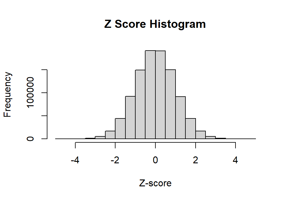

plot(density(Normal.Sample.Z),
  main="Probability Density Function", 
  xlab="z-score", ylab="Probability", 
  xlim=c(-3.25, 3.25))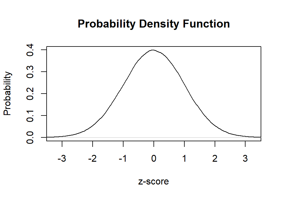

• Look a the PDF in your book and you will this matches. Lets put all into practice!

Why You Need to Standardize

Imagine you are teaching 3 classes: Statistics, Cognition, & Neuro. You have a student in all three classes, and she wants to how to compare her exam scores between all three classes (with N = 50 in each; but this does not need to be the case).

Student scores:

• Stats: \(X = 40\)
• Cog: \(X = 83\)
• Neuro: \(X = 60\)

Black line = Student score relative to the class

set.seed(123)
N=50
Stats.class<-rnorm(N, mean=60,sd=8)
hist(Stats.class,
  main="Raw Score Histogram", 
  xlab="Stats Exam", ylab="Frequency")
abline(v=40, col="red")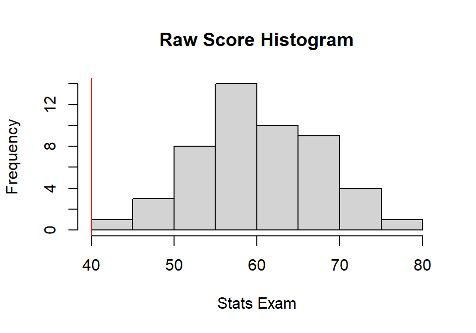

Stats.Mean<-mean(Stats.class)
Stats.sd<-sd(Stats.class)

set.seed(123)
N=50
Cognition<-rnorm(N, mean=75,sd=4)
hist(Cognition,
  main="Raw Score Histogram", 
  xlab="Cognitive Exam", ylab="Frequency")
abline(v=83, col="black")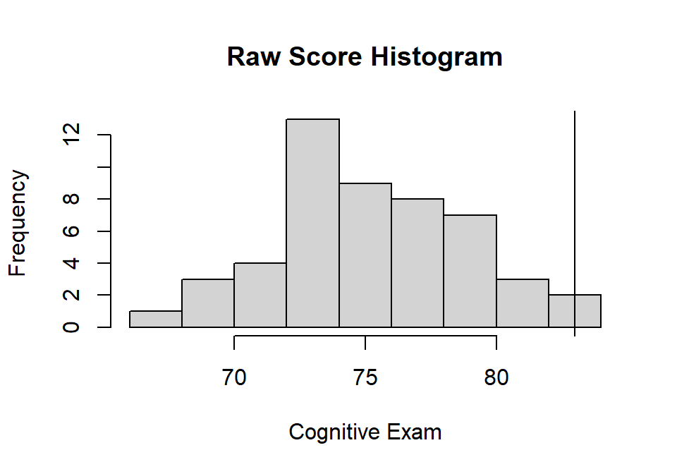

Cog.Mean<-mean(Cognition)
Cog.sd<-sd(Cognition)

set.seed(123)
N=50
Neuro<-rnorm(N, mean=40,sd=15)
hist(Neuro,
  main="Raw Score Histogram", 
  xlab="Neuro Exam", ylab="Frequency")
abline(v=60, col="black")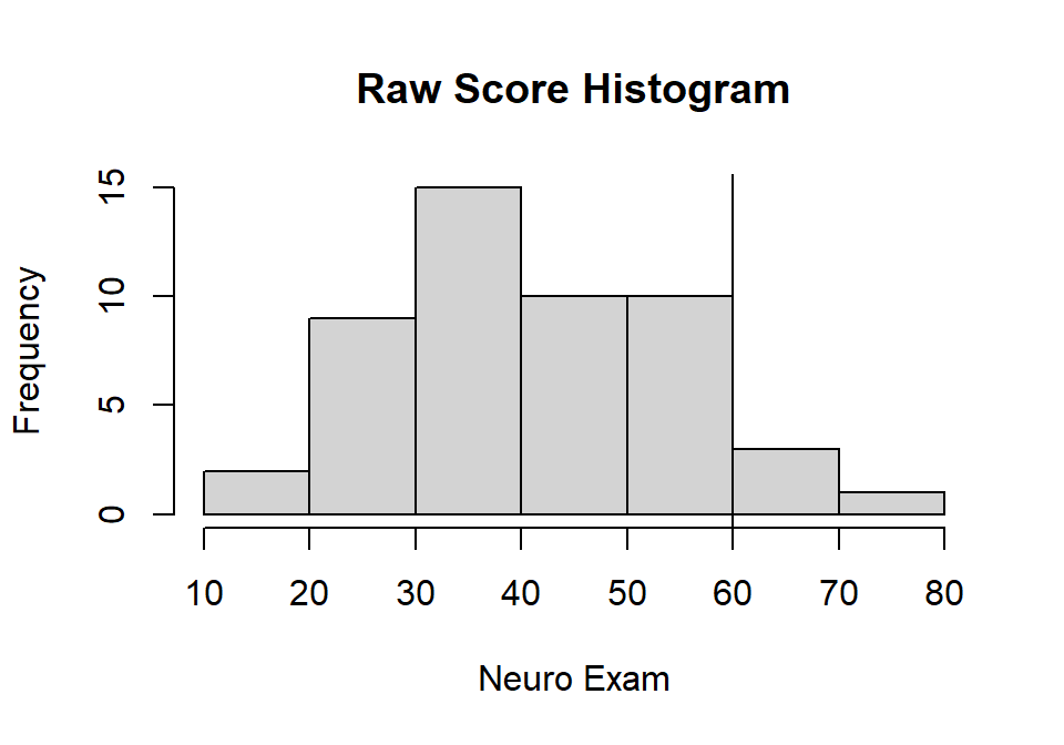

Neuro.Mean<-mean(Neuro)
Neuro.sd<-sd(Neuro)

Course Descriptive

• Stats: M = 60.275, sd = 7.407
• Cog: M = 75.138, sd = 3.703
• Neuro: M = 40.516, sd = 13.888

The student looks at the histograms and the class mean/sd and says so what? [Now you know why they failed your stats exam]

Find Percentile

• We need the z-score for the individual score, so we will use the sample zscore formula to calculate their individual zscore by hand

\[Z = \frac{X - M}{s}\]

Z-Scores per Exam

Stats.Z<-(40 - mean(Stats.class))/sd(Stats.class)
Cog.Z<-(83 - mean(Cognition))/sd(Cognition)
Neuro.Z<-(60 - mean(Neuro))/sd(Neuro)

• Stats: Z = -2.737
• Cog: Z = 2.123
• Neuro: Z = 1.403

Student says so what does all this mean?

Let’s assume the normal distribution and give them their percentile

Relative the normal distribution here is how the three tests are

plot(density(Normal.Sample.Z),
  main="Probability Density Function", 
  xlab="z-score", ylab="Probability", 
  xlim=c(-3.25, 3.25))
abline(v=Stats.Z, col="red")
abline(v=Cog.Z, col="blue")
abline(v=Neuro.Z, col="green")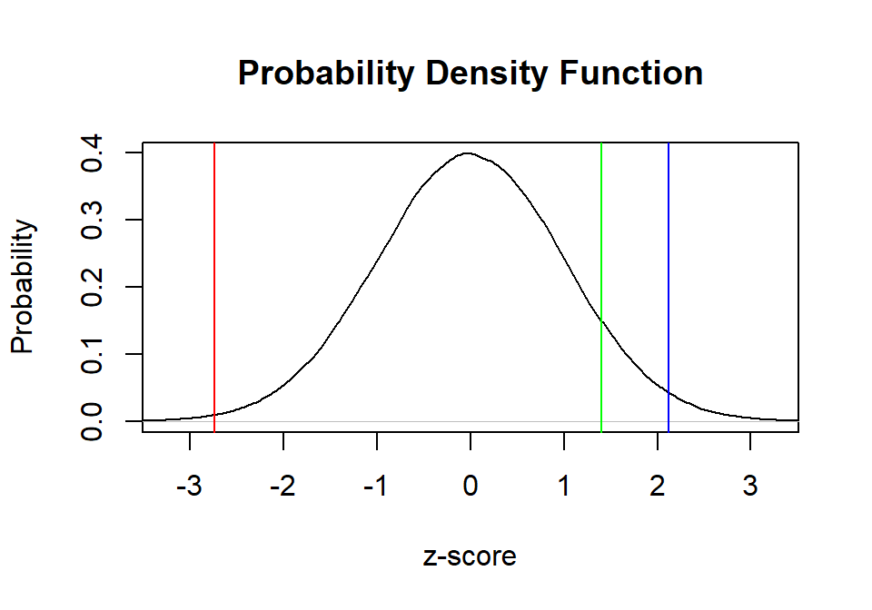

The percentile can be easier seen in the CDF of these positions. We can do that via the ecdf function (which is slow). The area under the curve behind the line percentile score can be calculated manually in R, but that is a slow process. R can look up those values for you with the function pnorm.

plot(ecdf(Normal.Sample.Z),
  main="Cumulative Density Function", 
  xlab="z-score", ylab="Probability", 
  xlim=c(-3.25, 3.25))
abline(v=Stats.Z, col="red")
abline(v=Cog.Z, col="blue")
abline(v=Neuro.Z, col="green")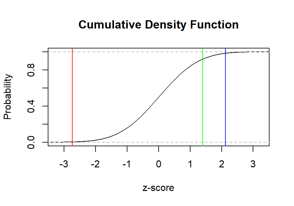

But wait? Do we assume the true population distribution of our sample is normal, or should we calculate the percentile for this data based on this distribution (empirically)? Mostly we assume the normal distribution and we use the tables in our book. Also, doing it empirically opens up a lot questions we will hold off for now.

Stats.Perc<-round(pnorm(Stats.Z)*100,1)
Cog.Perc<-round(pnorm(Cog.Z)*100,1)
Neuro.Perc<-round(pnorm(Neuro.Z)*100,1)

• Stats: Percentile = 0.3
• Cog: Percentile = 98.3
• Neuro: Percentile = 92

Check this numbers in your tables!

You tell the student they need to start doing their stats homework!

Sampling Error

We rarely, if ever, get to work with population data. Instead, we sample our population and hope we can estimate the parameters of the population distribution via sample statistics. In R, we can simulate this process very quickly.

Sample

To extract a sample in R from a population, we can do it a few ways. However, we will do it the more verbose way for now (but it is slower to run).

Step 1: Generate/View population

We did this way before using our the rnorm function. Here is the histogram again:

hist(Normal.Sample.1,
  main="Raw Score Histogram", 
  xlab="Population Distribution", ylab="Frequency")
abline(v=100, col="black")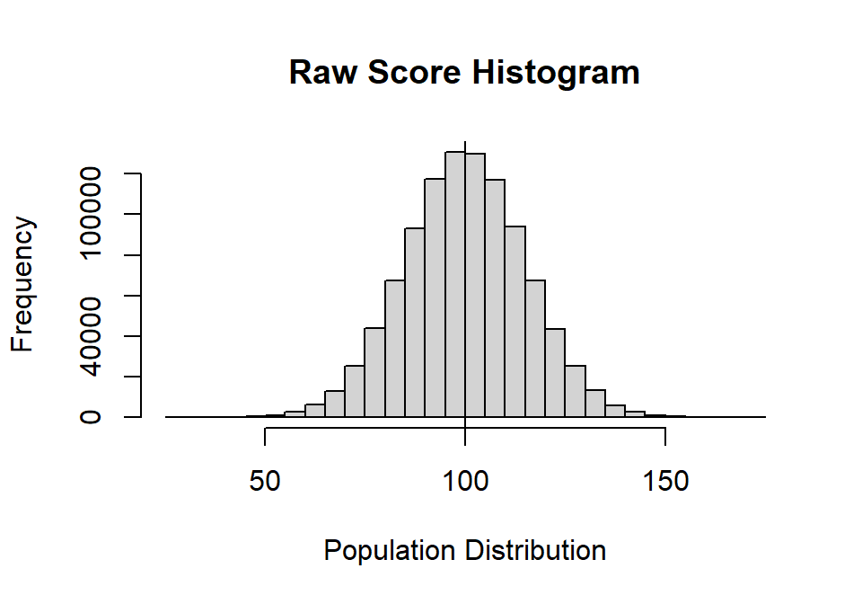

Step 2: Randomly sample from the distribution

We can use the sample function. The function works as follows: sample(distro, sample size you want, with/without replacement). If you ?sample, you will notice the default is to sample without replacement, so we need to override that argument. Note: We again need to set a seed to get the same answer

set.seed(42)
SampleSize = 10
sample.1<-sample(Normal.Sample.1, SampleSize, replace = TRUE)

hist(sample.1,
  main="Raw Score Histogram", 
  xlab="Sample Distribution", ylab="Frequency")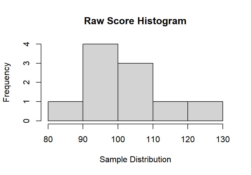

Step 3: Calculate moments of sample

M.1<-mean(sample.1)
SD.1<-sd(sample.1)
SK.1<-skewness(sample.1)
K.1<-kurtosis(sample.1)-3

Moments	M	S	Skewness	Kurtosis
Pop Params	100	15	0	0
Sim moments	99.99	14.99	0	-0.15
Sample moments	100.18	12.06	0.59	-0.15

You can see how our moments of the sample are different from our population (sampling error)

Step 4: Simulate 1000 samples!

The replicate function allows us to sample over and over again (creating a matrix of 10 values per sample X 1000 samples). The apply function allows us to apply a function across rows or columns (we want to apply over columns as each column is a sample).

NumberofSamples=1000
SampleSize=10
Sample.Results<-replicate(NumberofSamples,sample(Normal.Sample.1, size = SampleSize, replace=TRUE))
Sample.Means<-apply(Sample.Results,2,mean)
Sample.SD<-apply(Sample.Results,2,sd)
Sample.SK<-apply(Sample.Results,2,skewness)
Sample.K<-apply(Sample.Results,2,kurtosis)-3

hist(Sample.Means,
  main="Means of Samples Histogram", 
  xlab="Means Distribution", ylab="Frequency")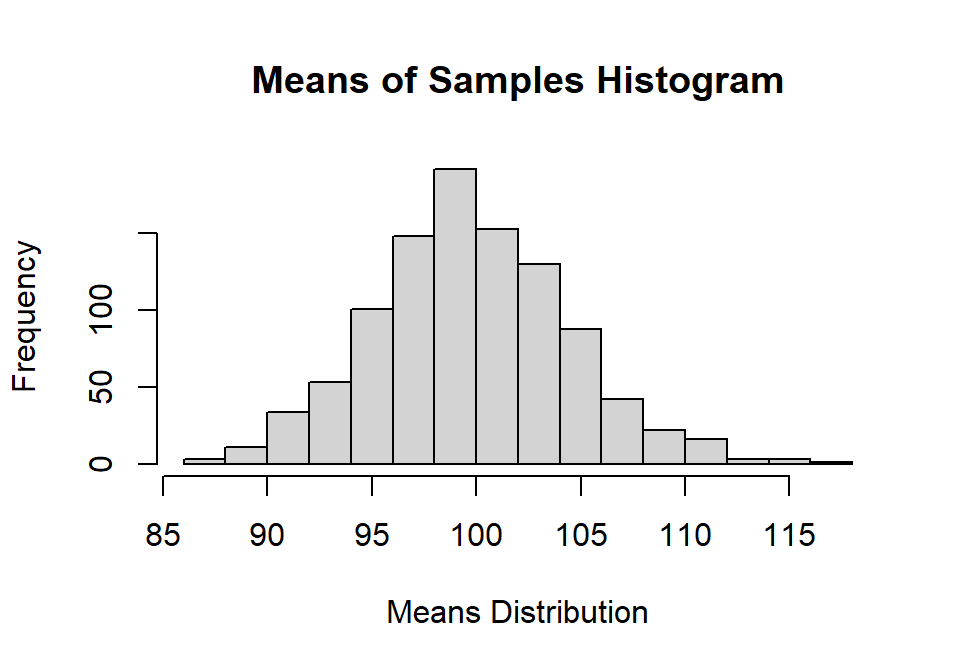

You will notice the distribution of means is normal and centered around 100, and it was precisely: Mean of means = 99.79 [very close to population!]

hist(Sample.SD,
  main="SD of Samples Histogram", 
  xlab="SD Distribution", ylab="Frequency")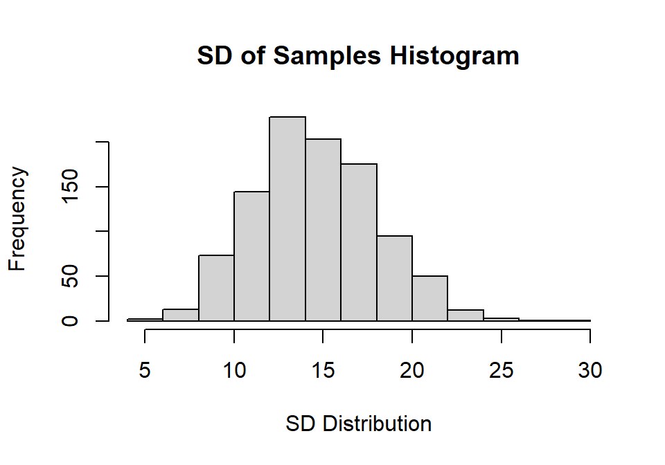

You will notice the distribution of SD is skewed a bit positive centered below around 15. Mean of SD = 14.55 [below our population as our sample size is small, so its biased estimate).

hist(Sample.SK,
  main="Skewness of Samples Histogram", 
  xlab="Skewness Distribution", ylab="Frequency")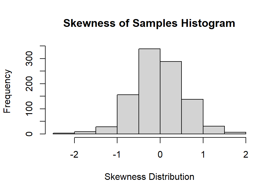

You will notice the distribution of skewness is skewed a bit as well centered around 0. Mean of skewness = -0.03

hist(Sample.K,
  main="Kurtosis of Samples Histogram", 
  xlab="Kurtosis Distribution", ylab="Frequency")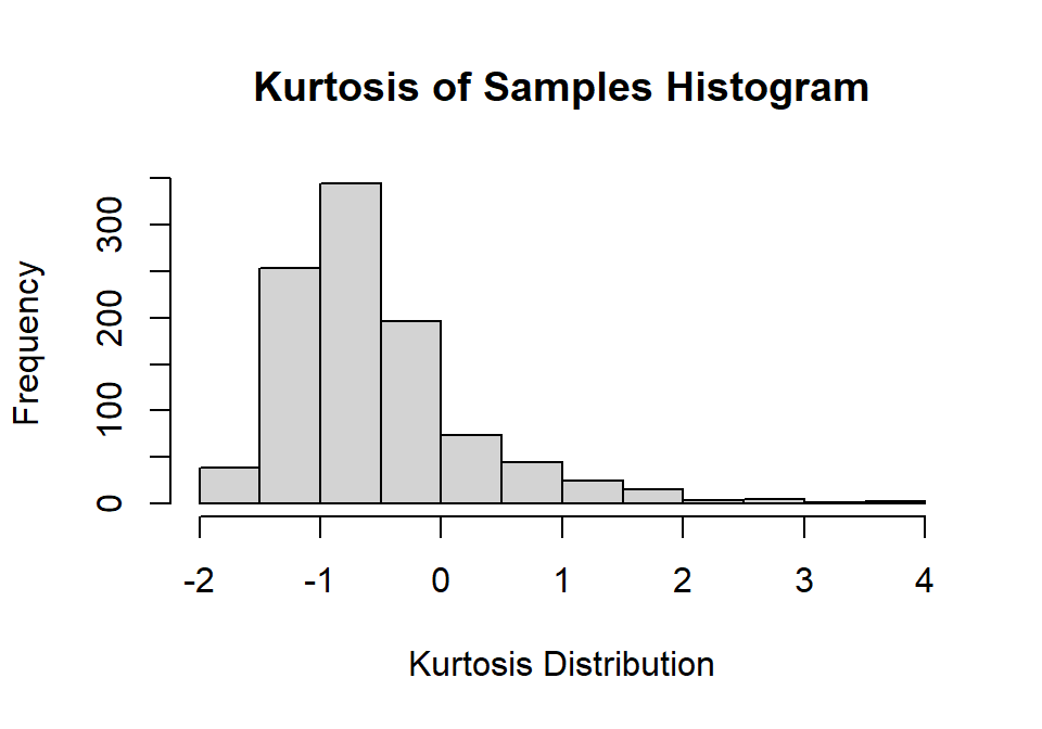

You will notice the distribution of kurtosis is very negatively skewed and not centered at zero. Mean of kurtosis = -0.56. Estimating the kurtosis is very difficult in small samples, and you will often have to assume you are working from a normal sample. If your sample size per study was larger, this would work much better.

Step 4: Moments of the Distribution of Means

Classical methods often use sample means to compare differences, as in the like the t-test and ANOVA (and not sd). We can thus extract our sampling error by examining the second moment of the distribution of means:

\[SE = \sqrt{\frac{\Sigma (M-M_{Grand})^2}{N-1}}\]

M.S<-mean(Sample.Means)
SD.S<-sd(Sample.Means)

The grand mean \(M_G\) = 99.79

Sampling error (spread of that mean) = 4.67

Standard Error

We cannot run thousands of samples, so we can approximate this value

\[SE = \frac{S}{\sqrt{N}}\]

So our first sample sd = 12.06 and it would estimate our standard error of the mean to be SE = 3.81, which is smaller but not too far from our simulated value. This value will be more accurate as our N increase, and our SD estimate gets more precise and accurate.

In fact, I can show how unstable the SE guess would actually be from our N = 10 simulation done 1000 times

SEM<-Sample.SD/SampleSize^.5

hist(SEM,
  main="SEM of Samples Histogram", 
  xlab="SEM Distribution", ylab="Frequency")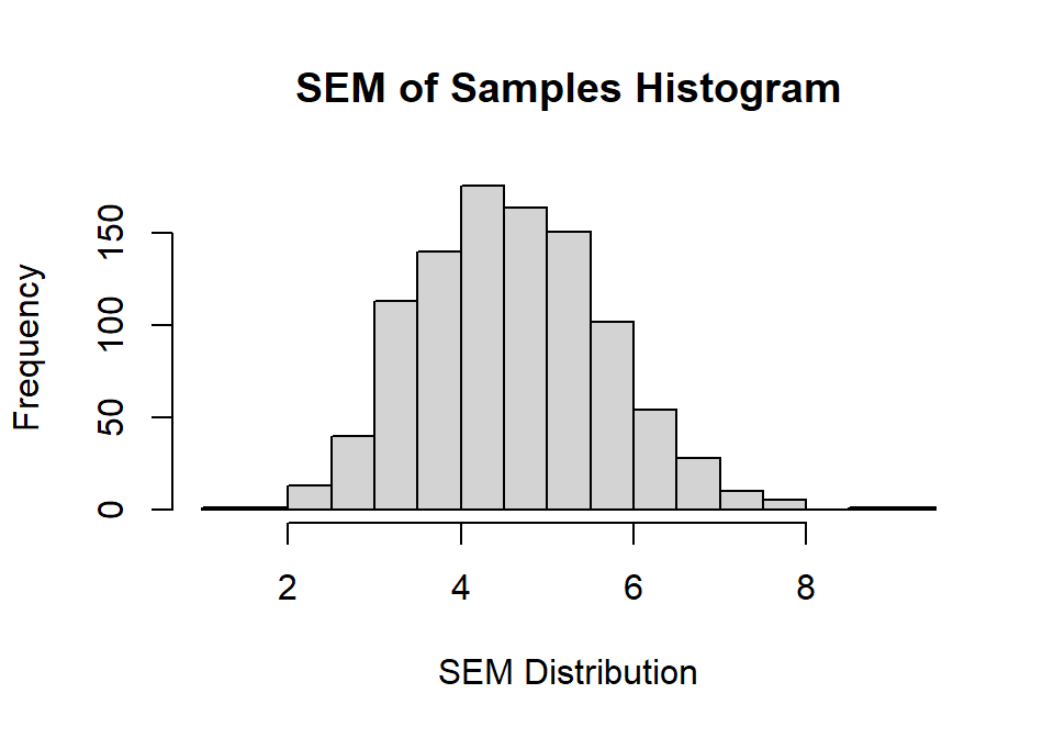

SEM.Estimate<-mean(SEM)

So our mean of the SE calculated values, mean SEM = 4.6 from our simulation is extremely close (but still smaller) than estimate our standard error of the SE from our simulation = 4.67. You will notice the distribution of possible SEM we could get from our studies is very large, and that is because our sample was very small. As you increase the sample size this distribution will narrow.

The main point is that samples are guesses of the population, and your guess will depend on the spread of the original distribution. The wider that distribution that larger the sample needs to be to estimate it. You cannot know if you are right, so we hope those numbers will replicate. If you reran the study and found the first two moments are jumping around, you probably need a much large sample size.