Missing Data

Missingness

Why is it missing?

• MCAR (Missing Completely At Random): “There’s no relationship between whether a data point is missing and any values in the data set, missing or observed.”

• MAR (Missing At Random): “means the propensity for a data point to be missing is not related to the missing data, but it is related to some of the observed data”. In other words, the response is missing because of another question you asked. You asked me if I like spiders, I said no. Next you ask me if I have a pet spider. I dont respond.

• MNAR (Missing Not At Random): “means the propensity for a data point to be missing is related to the missing data”. You have no idea why the response/question is missing, thus you cannot infer it.

Best MCAR. Worst is MNAR.

• See: http://www.theanalysisfactor.com/mar-and-mcar-missing-data/
• See: https://www.r-bloggers.com/imputing-missing-data-with-r-mice-package/

How big is my data set

• Normal to Huge data set: Losing 5-10% of your data is not a problem. Move on in life. If larger, then you have to start thinking about missing analysis and replacement.
• Very small data set (5-10 people per IV): Tea leaf reading or voodoo.

Common methods to Impute Missing data

• Impute: “assign (a value) to something by inference from the value of the products or processes to which it contributes”.

Classical Methods (assumining MCAR)

• Listwise deletion: Removes whole subject if one data point is missing. Easy to implement, but loses alot of data.

• Pairwise deletion: Removes just that case of that subjects data (keeps most data). Can be to implement (can mess up the error term or make DF differ from model to model), but less data is lost.

• Mean imputation: Fill in the missing data points with the mean of that variable. Lowers variance overall and keeps subject. No data loss, but you are affecting the error term and keeping the DF. This can create problems in very small samples.

• Conditional mean imputation: Replaces missing values with the predicted scores from a linear regression equation. [Very complicated when MAR is an issue]

• Most common in psychology tend to be Mean or Pair- or listwise (SPSS defaults depending on analysis. R defaults to listwise in most cases)

• For a review of the theory see: Peugh, J. L., & Enders, C. K. (2004). Missing data in educational research: A review of reporting practices and suggestions for improvement. Review of Educational Research, 74, 525-556.

Classical Methods

• We will do the listwise and mean replacement types
• Simulate a simple regression - remove cases completely at random and test

Typical Sample Size

• Simulate a data set

library(car)
set.seed(42)
n <- 50
# IVs
X <- runif(n, -10, 10)
Z <- rnorm(n, -10, 10)
# Our equation to  create Y
Y <- .8*X - .4*Z + 2 + rnorm(n, sd=10)
#Built our data frame
DataSet1<-data.frame(DV=Y,IV1=X,IV2=Z)

• Remove IVs and DVs at random (ampute) at about 40% total across the IVs and DV

library(mice)
set.seed(666)
Amputed.Data<-ampute(data =DataSet1, prop = 0.4, mech = "MCAR")
DataSet1.M<-Amputed.Data$amp

• Lets visualize the missingness

library(VIM)
aggr(DataSet1.M, col=c('navyblue','red'), numbers=TRUE, 
     sortVars=TRUE, labels=names(data), cex.axis=.7, 
     gap=3, 
     ylab=c("Histogram of missing data","Pattern"))

## 
##  Variables sorted by number of missings: 
##  Variable Count
##       IV1  0.20
##       IV2  0.16
##        DV  0.14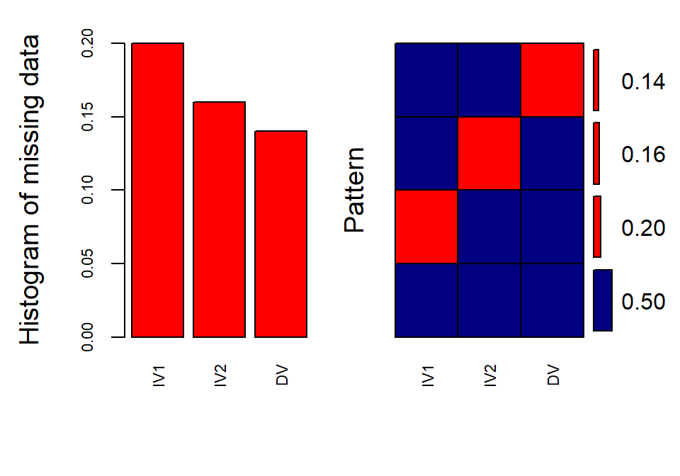

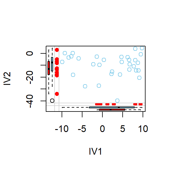
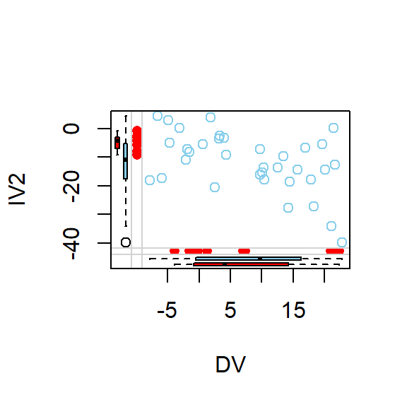
• Lets visualize pairwise scatterplots based on where the missing data seems to be

marginplot(DataSet1.M[c(1,2)])
marginplot(DataSet1.M[c(2,3)])
marginplot(DataSet1.M[c(1,3)])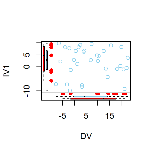

• Run the regression of the original and missing data side by side
• R defaults to listwise deletion (most conservative approach)
• Pairwise-deletion regression is not build into R by default (but there is is pairwise deletion for other methods)
• Original, Listwise, mean imputed (using the mice package)
  • Note: The function complete is in multiple packages (tidyr and mice) and they conflict, so I will use mice::complete to tell R which complete I want)

Orginal<-lm(DV~IV1+IV2, data= DataSet1)
Listwise<-lm(DV~IV1+IV2, data= DataSet1.M)

# Mean impute using MICE 
DataSet1.MM<- mice::complete(mice(DataSet1.M, meth='mean',printFlag = FALSE))
MeanImpute<-lm(DV~IV1+IV2, data= DataSet1.MM)

	Dependent variable:
	DV
	Orginal	Listwise	Mean Impute
	(1)	(2)	(3)
Constant	2.612 (1.909)	3.164 (2.665)	3.402 (1.846)
IV1	0.133 (0.209)	0.017 (0.276)	-0.056 (0.216)
IV2	-0.428** (0.131)	-0.361 (0.174)	-0.428** (0.131)
Observations	50	25	50
R2	0.192	0.165	0.186
Adjusted R2	0.158	0.089	0.151
F Statistic	5.590** (df = 2; 47)	2.169 (df = 2; 22)	5.373** (df = 2; 47)
Note:	p<0.05; p<0.01; p<0.001

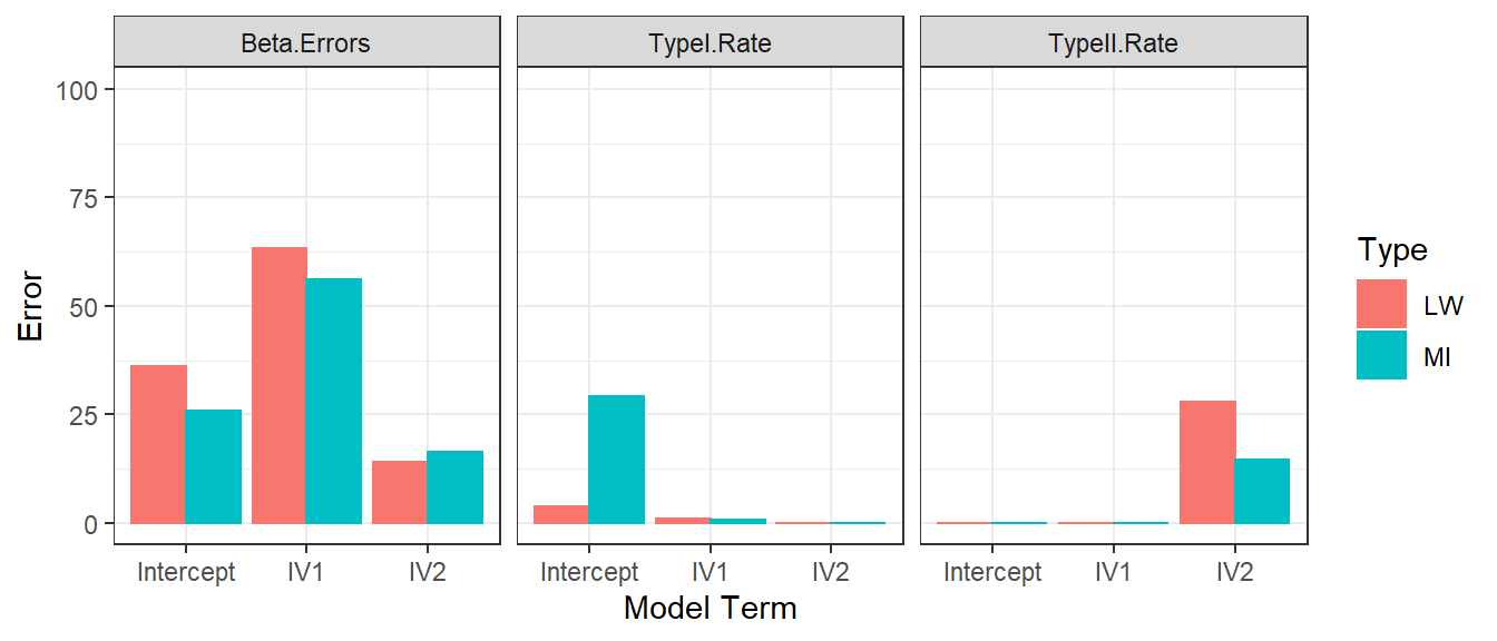
• If we run 1000 simulations for each methods, we can get an estimate of there Error
  • Betas for each parameter in the model (Estimated b - Orginal b/Orginal b)
    • We will take the median across simulations
  • Decisions errors using significance [Type I and Type II]
    • Type I = Orginal is not sig, but estimated is sig
    • Type II = Orginal is sig, but estimated is not sig
    • Look to the “orginal” simulation table to see which is possible for that model term

Huge Data Set

• N = 500

set.seed(42)
n <- 500
# IVs
X <- runif(n, -10, 10)
Z <- rnorm(n, -10, 10)
# Our equation to  create Y
Y <- .8*X - .4*Z + 2 + rnorm(n, sd=10)
#Built our data frame
DataSet2<-data.frame(DV=Y,IV1=X,IV2=Z)
#remove cases at random 
set.seed(666)
Amputed.Data.2<-ampute(data =DataSet2, prop = 0.4, mech = "MCAR")
DataSet2.M<-Amputed.Data.2$amp

Orginal.2<-lm(DV~IV1+IV2, data= DataSet2)
Listwise.2<-lm(DV~IV1+IV2, data= DataSet2.M)
# Mean impute using MICE 
DataSet2.MM<- mice::complete(mice(DataSet2.M, meth='mean',printFlag = FALSE))
MeanImpute.2<-lm(DV~IV1+IV2, data= DataSet2.MM)

	Dependent variable:
	DV
	Orginal	Listwise	Mean Impute
	(1)	(2)	(3)
Constant	2.249** (0.680)	2.439** (0.932)	3.254*** (0.694)
IV1	0.817*** (0.079)	0.858*** (0.107)	0.710*** (0.084)
IV2	-0.378*** (0.047)	-0.352*** (0.066)	-0.274*** (0.050)
Observations	500	303	500
R2	0.258	0.231	0.170
Adjusted R2	0.255	0.226	0.167
F Statistic	86.263*** (df = 2; 497)	44.974*** (df = 2; 300)	50.876*** (df = 2; 497)
Note:	p<0.05; p<0.01; p<0.001

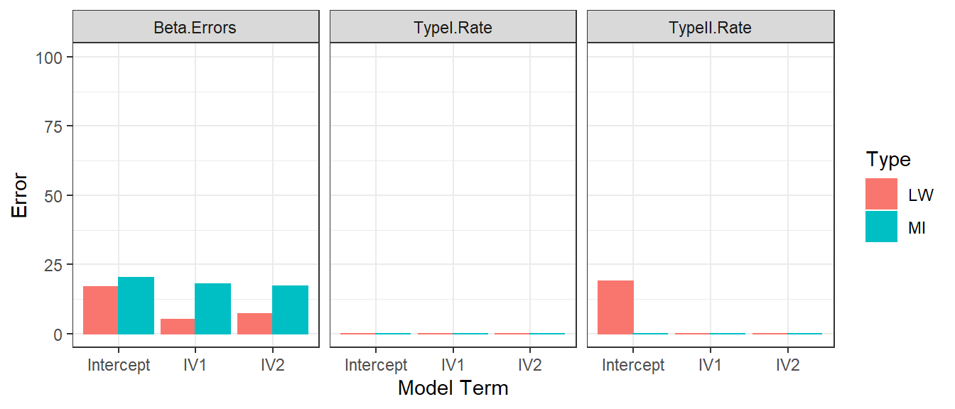
• We repeat the Error simulations for each methods using 500 subjects

Tiny Sample Size

• N = 15

set.seed(42)
n <- 15
# IVs
X <- runif(n, -10, 10)
Z <- rnorm(n, -10, 10)
# Our equation to  create Y
Y <- .8*X - .4*Z + 2 + rnorm(n, sd=10)
#Built our data frame
DataSet3<-data.frame(DV=Y,IV1=X,IV2=Z)

#remove cases at random 
set.seed(666)
Amputed.Data.3<-ampute(data =DataSet3, prop = 0.4, mech = "MCAR")
DataSet3.M<-Amputed.Data.3$amp

Orginal.3<-lm(DV~IV1+IV2, data= DataSet3)
Listwise.3<-lm(DV~IV1+IV2, data= DataSet3.M)

# Mean impute using MICE 
DataSet3.MM<- mice::complete(mice(DataSet3.M, meth='mean',printFlag = FALSE))
MeanImpute.3<-lm(DV~IV1+IV2, data= DataSet3.MM)

	Dependent variable:
	DV
	Orginal	Listwise	Mean Impute
	(1)	(2)	(3)
Constant	3.822 (3.024)	3.259 (5.843)	1.427 (3.031)
IV1	1.310* (0.526)	0.802 (1.110)	1.124 (0.575)
IV2	-0.225 (0.272)	0.105 (0.854)	-0.603* (0.263)
Observations	15	8	15
R2	0.405	0.127	0.373
Adjusted R2	0.306	-0.222	0.268
F Statistic	4.081* (df = 2; 12)	0.364 (df = 2; 5)	3.565 (df = 2; 12)
Note:	p<0.05; p<0.01; p<0.001

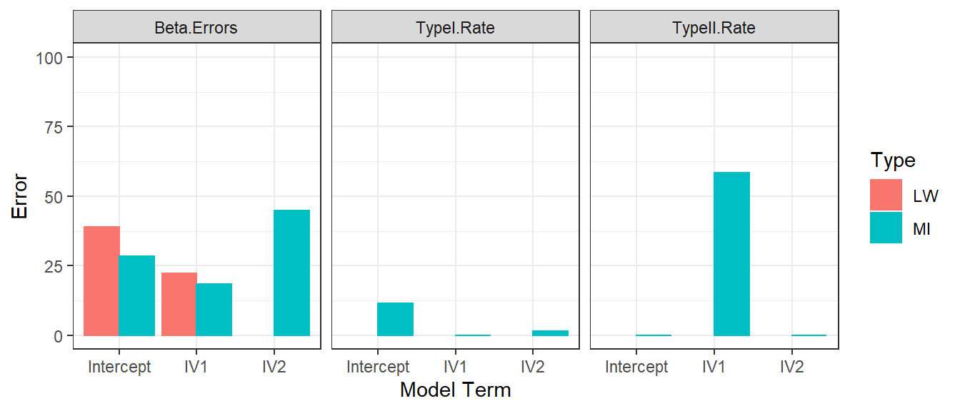
• We repeat the Error simulations for each methods using 15 subjects

Typical Samples with MNAR

• N = 50

#remove cases at random from our orginal data set
set.seed(666)
Amputed.Data.4<-ampute(data =DataSet1, prop = 0.4, mech = "MNAR")
DataSet4.M<-Amputed.Data.4$amp

Orginal.4<-lm(DV~IV1+IV2, data= DataSet1)
Listwise.4<-lm(DV~IV1+IV2, data= DataSet4.M)
# Mean impute using MICE 
DataSet4.MM<- mice::complete(mice(DataSet4.M, meth='mean',printFlag = FALSE))
MeanImpute.4<-lm(DV~IV1+IV2, data= DataSet4.MM)

	Dependent variable:
	DV
	Orginal	Listwise	Mean Impute
	(1)	(2)	(3)
Constant	2.612 (1.909)	1.368 (2.277)	1.948 (1.708)
IV1	0.133 (0.209)	0.133 (0.266)	0.096 (0.197)
IV2	-0.428** (0.131)	-0.421* (0.155)	-0.388** (0.118)
Observations	50	30	50
R2	0.192	0.222	0.189
Adjusted R2	0.158	0.164	0.154
F Statistic	5.590** (df = 2; 47)	3.851* (df = 2; 27)	5.468** (df = 2; 47)
Note:	p<0.05; p<0.01; p<0.001

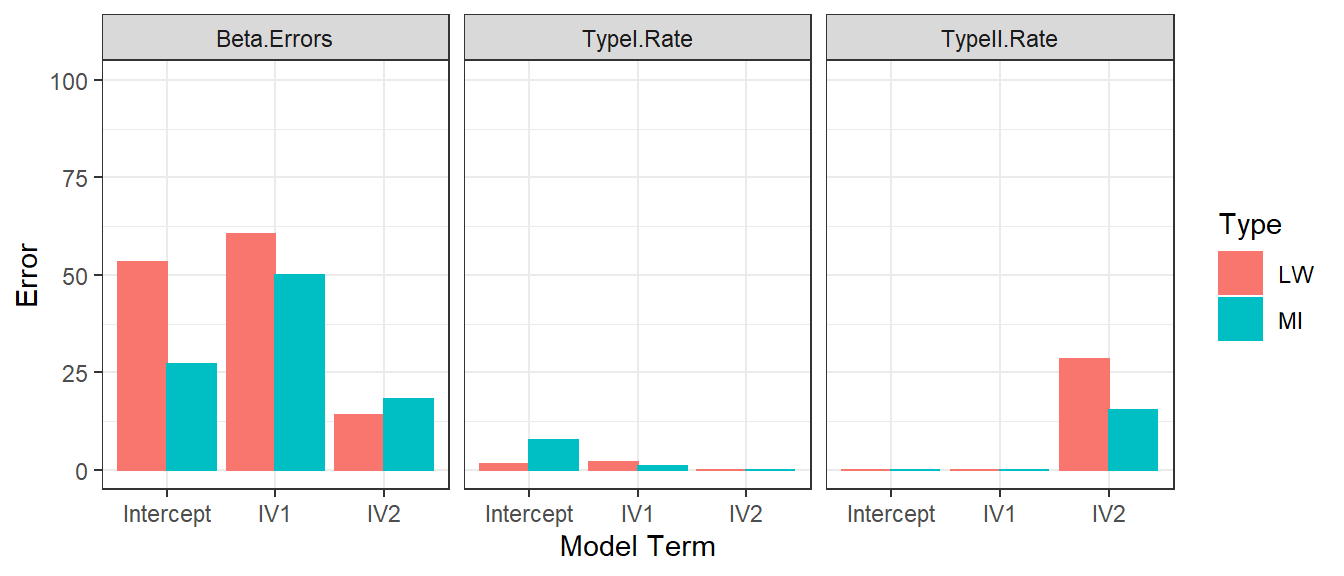
• We repeat the Error simulations for each methods for MNAR (50 subjects)

Typical Samples with MAR

• N = 50

#remove cases from our orginal data set
set.seed(42)
Amputed.Data.5<-ampute(data =DataSet1, prop = 0.4, mech = "MAR")
DataSet5.M<-Amputed.Data.5$amp

Orginal.5<-lm(DV~IV1+IV2, data= DataSet1)
Listwise.5<-lm(DV~IV1+IV2, data= DataSet5.M)
# Mean impute using MICE 
DataSet5.MM<- mice::complete(mice(DataSet5.M, meth='mean',printFlag = FALSE))
MeanImpute.5<-lm(DV~IV1+IV2, data= DataSet5.MM)

	Dependent variable:
	DV
	Orginal	Listwise	Mean Impute
	(1)	(2)	(3)
Constant	2.612 (1.909)	0.863 (2.265)	2.996 (1.915)
IV1	0.133 (0.209)	0.134 (0.228)	0.011 (0.216)
IV2	-0.428** (0.131)	-0.439** (0.141)	-0.422** (0.133)
Observations	50	34	50
R2	0.192	0.244	0.176
Adjusted R2	0.158	0.195	0.141
F Statistic	5.590** (df = 2; 47)	5.000* (df = 2; 31)	5.023* (df = 2; 47)
Note:	p<0.05; p<0.01; p<0.001

• We repeat the Error simulations for each methods for MAR (50 subjects)

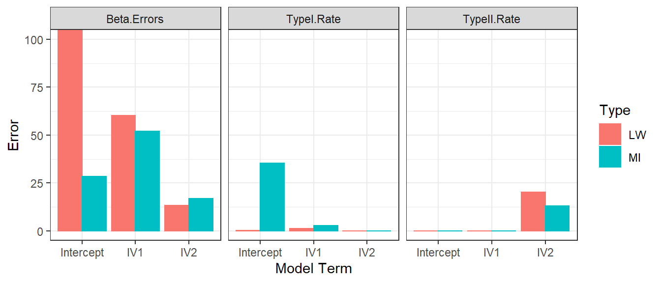
Notes

• Mean imputing works OK in medium to large sample sizes
• But it creates large bias in small samples
• If you don’t have MCAR you have to turn to more complex methods

Modern approaches

• There are many modern approaches often based on maximum likelihood estimation (ML) or Multiple Imputation (MI) or even Bayesian approaches
• “ML estimation is to identify the population parameter values most likely to have produced a particular sample of data. This usually requires an iterative process whereby the model fitting program”tries out” different values for the parameters of interest (e.g., regression coefficients) en route to identifying the values most likely to have produced the sample data.” (Peugh & Enders, 2004)
• Multiple Imputation: “Rather than treating a single set of imputed values as”true” estimates of the missing values, MI creates a number of imputed data sets (frequently between 5 and 10), each of which contains a different plausible estimate of the missing values.” (Peugh & Enders, 2004)
• Lets test out MI as its the newest and considered an improvement over ML

Multiple Imputation by Chained Equations

• See Azur et al, 2011 for details
• MICE package in R: Lots of old and modern algorithms to choose from (also for design beyond linear regression)
• Predictive mean matching is a good version to use as it “is a general purpose semi-parametric imputation method. … imputations are restricted to the observed values and that it can preserve non-linear relations…” (Buuren & Groothuis-Oudshoorn, 2011)
• We will work from our MAR missing Dataset5.M
• We can compare this to our classical methods and some other methods which the package allows (Bootstapping & Bayesian)

Typical sample size

#Linear regression using bootstrap
DataDataSet5.Boot<- mice::complete(mice(DataSet5.M, m = 10,meth='norm.boot',
                                  printFlag = FALSE, seed = 666))
Boot<-lm(DV~IV1+IV2, data= DataDataSet5.Boot)

#Bayesian linear regression
DataDataSet5.BLR<- mice::complete(mice(DataSet5.M, m = 10,meth='norm',
                                 printFlag = FALSE, seed = 666))
BLR<-lm(DV~IV1+IV2, data= DataDataSet5.BLR)

#Predictive mean matching 
DataDataSet5.pmm<- mice::complete(mice(DataSet5.M, m = 10,meth='pmm',
                                 printFlag = FALSE, seed = 666))
PMM<-lm(DV~IV1+IV2, data= DataDataSet5.pmm)

	Dependent variable:
	DV
	Orginal	Boot	BLR	PMM
	(1)	(2)	(3)	(4)
Constant	2.612 (1.909)	0.531 (1.889)	-0.099 (1.817)	1.355 (1.779)
IV1	0.133 (0.209)	-0.011 (0.210)	-0.007 (0.191)	0.002 (0.206)
IV2	-0.428** (0.131)	-0.551*** (0.117)	-0.546*** (0.104)	-0.478*** (0.108)
Observations	50	50	50	50
R2	0.192	0.325	0.377	0.295
Adjusted R2	0.158	0.296	0.351	0.265
F Statistic (df = 2; 47)	5.590**	11.289***	14.247***	9.835***
Note:	p<0.05; p<0.01; p<0.001

• Predictive mean matching is the default of this program and you see it does a good job

Small sample size

• Use the same exact small data (N = 15)

#Linear regression using bootstrap
DataDataSet3.Boot<- mice::complete(mice(DataSet3.M, m = 15,meth='norm.boot',
                                  printFlag = FALSE, seed = 666))
Boot.3<-lm(DV~IV1+IV2, data= DataDataSet3.Boot)

#Bayesian linear regression
DataDataSet3.BLR<- mice::complete(mice(DataSet3.M, m = 15,meth='norm',
                                 printFlag = FALSE, seed = 666))
BLR.3<-lm(DV~IV1+IV2, data= DataDataSet3.BLR)

#Predictive mean matching 
DataDataSet3.pmm<- mice::complete(mice(DataSet3.M, m = 15,meth='pmm',
                                 printFlag = FALSE, seed = 666))
PMM.3<-lm(DV~IV1+IV2, data= DataDataSet3.pmm)

	Dependent variable:
	DV
	Orginal	Boot	BLR	PMM
	(1)	(2)	(3)	(4)
Constant	3.822 (3.024)	0.978 (3.532)	-0.047 (4.002)	4.401 (4.016)
IV1	1.310* (0.526)	0.741 (0.683)	1.192 (0.756)	1.038 (0.670)
IV2	-0.225 (0.272)	-0.800 (0.397)	-0.489 (0.317)	-0.441 (0.339)
Observations	15	15	15	15
R2	0.405	0.265	0.219	0.213
Adjusted R2	0.306	0.142	0.088	0.082
F Statistic (df = 2; 12)	4.081*	2.161	1.679	1.621
Note:	p<0.05; p<0.01; p<0.001

• We need to find practicer of the dark arts, as none of the methods did a good job

Notes

• You have to manually set the number of iterations (number of passes)
• You will have to research each algorithm for your particular data missingness

Best Practices

• Each situation is different and which method you use depends on many factors
• Also you must think carefully about the assumptions you are making
• For example, if you mean (or PMM) replace you are assuming the data are normal
• There are other advanced methods for specific situation: “hot decking” for survey research; nearest neighbor, splines, or autoregressive methods for time-series or longitudinal data
• Best practice: compare serval logical replacement methods and also compare it to listwise removal. If the story you are trying to tell is very different based on each method and very different as it relates to the listwise removal it suggests you have not factored in some assumption correctly and best to rethink what you are doing.